If you want to implement Magic Kernel Sharp, jump straight to my instructions below, and feel free to contact me if you need help.
This paper (62 pages) provides a full mathematical analysis of Magic Kernel Sharp and shows why it is superior to the Lanczos kernels:
It is heavy, but thorough, and has nice images and graphs. There was some discussion of it on Hacker News and its Facebook Page.
“The magic kernel” is, today, a colloquial name for Magic Kernel Sharp, the world’s gold standard image resizing algorithm that powers all the images on Facebook and Instagram and has almost universally replaced the previous gold standard Lanczos kernels. Resized images are crystal clear and astoundingly free of the artifacts that all other algorithms produce, no matter how large the enlargement or how small the reduction. Best of all, Magic Kernel Sharp is actually more computationally efficient than the Lanczos kernels.
I originally came across what I dubbed at that time a “magic” kernel in 2006 in the source code for what is now the standard JPEG library. I found empirically that this “kernel”—in reality just interpolation weights of 1/4 and 3/4—allowed an image to be doubled in size, as many times as desired, astonishingly clearly. Experts pointed out, however, that the resulting images were slightly blurrier than an ideal resizer would produce.
In 2011 I investigated the remarkable properties of this “magic” kernel in depth, as a hobby, and generalized it to allow resizing an image to any arbitrary size—larger or smaller. I dubbed this generalization “the Magic Kernel.”
In early 2013, shortly after starting as a Software Engineer E6 at Facebook, I was working on a side project with fellow software engineer Kevin Dale to address quality problems with the back-end resizing of all photos uploaded to Facebook, and realized that adding a simple three-tap sharpening step to the output of an image resized with the Magic Kernel yielded a fast and efficient resizing algorithm with close to perfect fidelity. I implemented the new algorithm in the Facebook C++ codebase as “Magic Kernel Sharp.”
This “factorization” of the algorithm into two independent parts—the original Magic Kernel resizing step, plus a final Sharp step—not only made the algorithm more computationally efficient, but it also allowed me to make use of hardware acceleration libraries that provided only same-size filtering functions and non-antialiased resizing functions. As a consequence of these properties, by mid-2013 Kevin and I were able to deploy Magic Kernel Sharp to the back-end resizing of all images on Facebook, with not only better quality, but also greater CPU and storage efficiency, than the code stack it replaced. These were critical factors for code that has since been executed trillions of times. (Others who have implemented Magic Kernel Sharp since that time don’t have these severe performance constraints, and just implement it as a single kernel.)
In early 2015 I numerically analyzed the Fourier properties of the Magic Kernel Sharp algorithm, and discovered that it possesses high-order zeros at multiples of the sampling frequency, which explains why it produces such amazingly clear results: these high-order zeros greatly suppress any potential aliasing artifacts that might otherwise appear at low frequencies, which is most visually disturbing.
When later in 2015 another software engineer, Georges Berenger, sought to migrate Instagram across to Facebook’s back-end image resizing infrastructure, we realized that the existing Instagram stack provided more “pop” for the final image than what Magic Kernel Sharp produced. I realized that I could simply adjust the Magic Kernel Sharp code to include this additional sharpening as part of the Sharp step. This allowed us to deploy this “Magic Kernel Sharp+” to Instagram—again, with greater CPU and storage efficiency and higher quality and resolution than the code stack it replaced.
In 2021 I derived a small refinement to the 2013 version of Magic Kernel Sharp, which yielded a kernel that is still completely practical, but fulfills the theoretical spectral neutrality of the Sharp step to at least nine bits of accuracy. I called this update “Magic Kernel Sharp 2021,” and to avoid confusion started referring to the original Facebook and Instagram version as “Magic Kernel Sharp 2013.”
Most practical image resizing applications use Magic Kernel Sharp 2013 or 2021 or both. I describe below how to do that. There is no “right answer” as to which you should prefer. Visual quality and computational efficiency are maximized with the original 2013 version that Facebook and Instagram use, but it does slightly sharpen the image (indeed, as I noted above, Instagram even sharpens it a bit more). The 2021 version is more mathematically correct and spectrally flat, not sharpening the image to any appreciable degree, but this mathematical correctness brings with it more “Gibbs ringing” at sharp edges, and the algorithm is also less computationally efficient than the original 2013 version. My recommendation is that you should use the 2013 version unless you have a strong practical, legal, or ideological reason for preferring spectral flatness. Personally, I have found that the 2013 version works better for my edge detection algorithm, for which the extra Gibbs ringing of the 2021 version is more damaging, whereas the 2021 version works better for my mipmapping algorithm, for which the extra sharpening of the 2013 version leads to exaggerated contrast which can wash out some subtle details.
Following my creation of Magic Kernel Sharp 2021, I delved again into the mathematical properties of Magic Kernel Sharp. (You may skip the rest of this paragraph if you are not interested in this aspect.) I analytically derived the Fourier transform of the Magic Kernel in closed form, and found, incredulously, that it is simply the cube of the sinc function. This implies that the Magic Kernel is just the rectangular window function convolved with itself twice—which, in retrospect, is completely obvious. (Mathematically: it is a cardinal B-spline.) This observation, together with a precise definition of the requirement of the Sharp kernel, allowed me to obtain an analytical expression for the exact Sharp kernel, and hence also for the exact Magic Kernel Sharp kernel, which I recognized is just the third in a sequence of fundamental resizing kernels. These findings allowed me to explicitly show why Magic Kernel Sharp is superior to any of the Lanczos kernels. It also allowed me to derive further members of this fundamental sequence of kernels, in particular the sixth member, which has the same computational efficiency as Lanczos-3, but has far superior properties. These findings are described in detail in the research paper above.
On the rest of this page I provide a brief historical overview of the development of Magic Kernel Sharp, and describe how you can implement it yourself.
A free and open source reference ANSI C implementation of Magic Kernel Sharp is provided at the bottom of this page. It is supplied under the MIT-0 License. You likely won’t want to build and run this reference implementation, since it is now built into standard utilities like ImageMagick (which, somewhat ironically, Kevin and I used at Facebook in 2013 to test Magic Kernel Sharp against what at that time was the gold standard, the Lanczos-3 kernel), and Alain Viddeleer has recently created a simple C/C++ implementation of it which is much easier to work from than my reference implementation code. The only time you might want to run it is if you want to test your own implementation using my testing tool, in which case you can just compile, build, and run it without needing to look at the actual source code.
I am happy to help anyone implementing, using, or researching Magic Kernel Sharp. Feel free to contact me directly.
The unimportant prehistory of how I got into any image processing at all might be of interest to young software engineers, and is here.
By 2006 I was looking at the code of what at that time was still referred to as “the IJG JPEG library” (today it is the standard JPEG library). Standard JPEG compression stores the two channels of chrominance data at only half-resolution, i.e., only one Cr and one Cb value for every 2 x 2 block of pixels. In reconstructing the image, it is therefore necessary to “upsample” the chrominance channels back to full resolution. The simplest upsampling method is to simply replicate the value representing each 2 x 2 block of pixels into each of the four pixels in that block, called “nearest neighbor” upsampling (even though, in this case, the “neighbor” is just the single value stored for that 2 x 2 block). The IJG library used that method by default, but it also provided an optional mode called “fancy upsampling.” The following example shows the difference in the resulting reconstructions (note, particularly, the edges between red and black):
Nearest neighbor upsampling of chrominance channels

“Fancy” upsampling of chrominance channels
Intrigued, I examined the C source code for this “fancy” upsampling. To my amazement, I discovered that it was nothing more than a simple interpolation in each direction, with a weight of 3/4 to the nearer 2 x 2 block center and a weight of 1/4 to the farther 2 x 2 block center! An alternative way of looking at it is that it is a “kernel” with values {1/4, 3/4, 3/4, 1/4} in each direction (where, in this notation, the standard “replication” or “nearest neighbor” kernel is just {0, 1, 1, 0}).
Further intrigued, I decided to try this kernel out on all three channels (not just the chrominance channels) of a general (not JPEG-compressed) image, so that the result would be the image doubled in size in each direction. To my astonishment, I found that this kernel was apparently “magic”: it gave astoundingly good results for repeated enlargements, no matter how many times it was applied:
![]()
Original image

One doubling with the “magic” kernel

Two doublings with the “magic” kernel

Three doublings with the “magic” kernel
Likewise, applying it as a downsampling kernel yielded beautifully antialiased images:

New original image

One halving with the “magic” kernel

Two halvings with the “magic” kernel
![]()
Three halvings with the “magic” kernel
Note that, as described in the introduction above, all of these images are more blurred than they need to be. This is because the addition of the post-sharpening step in Magic Kernel Sharp was at this point in time still seven years in the future.
Being well versed in signal processing theory and aliasing artifacts, I could not understand how this “magic” kernel was providing such remarkable results.
Flabbergasted, and unable to find this kernel either in textbooks or on the web, I asked on the newsgroups whether it was well-known, headed by the subject line that heads this section (“ ‘Magic’ kernel for image zoom resampling?”): see here and here. It appeared that it was not.
The theoretically perfect antialiasing kernel is a sinc function. In practice, its infinite support necessitates approximations, such as the Lanczos kernels.
The question, then, was obvious: how on Earth could the simple kernel {1/4, 3/4, 3/4, 1/4} do such a good job when enlarging an image?
In 2006, the newsgroup discussions following my postings identified that the “magic” kernel is effectively a very simple approximation to the sinc function, albeit with the twist that the new sampling positions are offset by half a pixel from the original positions. (This is obvious when one considers the “tiling” of the original JPEG chrominance implementation, but it is not at all an obvious choice from the point of view of sampling theory.)
However, this didn’t really explain why it worked so well. There are many other approximations to the sinc function that do not do a very good job of antialiasing at all.
In any case, I simply put aside such theoretical questions, and made practical use of the “magic” kernel in a mipmapping (progressive download) method, which I dubbed JPEG-Clear.
Following my development of JPEG-Clear, my work on image processing went onto the backburner, as in 2007 I moved into a more challenging day job: developing and implementing algorithms for a private hedge fund.
The theoretical mystery of the “magic” kernel would remain for another five years.
By 2011, however, I had moved on again, and my day job was to process image and volumetric data for prostate cancer research. As part of that work I was looking at edge detection algorithms (to find the edge of the prostate).
I realized that I could use the “magic” kernel to create an edge detection operator that avoided some of the pitfalls of the standard methods.
My edge detection paper caught the attention of Charles Bloom, who dissected it in some detail, in particular the “magic” kernel. His discussion of the edge detector itself can be left to another place; but Bloom did note that the “magic” kernel can be factorized into a nearest-neighbor upsampling to the “doubled” (or “tiled”) grid, i.e. {1, 1}, followed by convolution with a regular {1/4, 1/2, 1/4} kernel in that new space.
This still didn’t explain why it did such an amazing job of upsizing and downsizing images, but it did rekindle my interest in exploring its properties.
Following Bloom’s factorization of the “magic” kernel, I started playing around with it again. I then discovered empirically that, when convolved with itself an arbitrary number of times, the resulting kernel was always piecewise parabolic—three separate parabolas joining together smoothly—allowing the kernel to “fit into itself” when convolved with a constant source signal (mathematically: it is a partition of unity; we will return to this below).
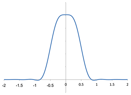
Taking this to its logical conclusion, I looked at what would happen if a signal were upsampled with the “magic” kernel an infinite number of times. If we denote by x the coordinate in the original sampled space (where the original signal is sampled at integral values of x), then, by nothing more than direct observation of the sequences of values produced, I deduced that the infinitely-upsampled Magic Kernel function is given analytically by
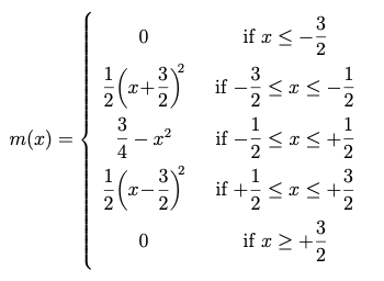
Analytical formula for the Magic Kernel
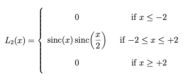
Here is a graph of m(x):
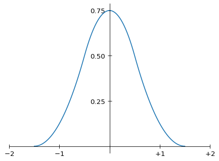
Graph of the Magic Kernel
Now, this doesn’t look much like a sinc function at all. So how and why does it work so well for enlarging an image?
Well, first, note that m(x) has finite support: a given sample of the original signal only contributes to the region from 1.5 spacings to the left to 1.5 spacings to the right of its position. This makes the kernel practical to implement.
Second, it’s convenient that m(x) is nonnegative. This avoids introducing “ringing,” and ensures that the output image has exactly the same dynamic range as the input image.
Third, m(x) is continuous and has continuous first derivative everywhere, including at the ends of its support. This property ensures that convolving with the Magic Kernel yields results that “look good”: discontinuities in the kernel or its first derivative—even at its endpoints—generally lead to artifacts (even if generally subtle) that may be detected by the human eye.
Fourth, m(x) is a partition of unity: it “fits into itself”; its being made up piecewise of three matching parabolas means that if we place a copy of m(x) at integral positions, and sum up the results, we get a constant (unity) across all x; the convex parabolas at the two ends match exactly the concave parabola in the middle:
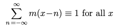
The partition of unity identity
This remarkable property can help prevent “beat” artifacts across a resized image.
Fifth, note that the shape of m(x) visually resembles that of a Gaussian, which (if one didn’t know anything about Fourier theory) would be the mathematician’s natural choice for an interpolation kernel. The standard deviation of m(x) can be calculated from the above functional form: it is 1/2. Comparing m(x) with a Gaussian with the same standard deviation shows that the resemblance is not just an illusion:
Comparing the Magic Kernel to a Gaussian
Remarkably, the seminal work in pyramid encoding in the early 1980s found exactly the same Gaussian-like properties for a five-tap filter with coefficients {0.05, 0.25, 0.4, 0.25, 0.05} (see here and here).
In contrast, a sinc function has oscillatory lobes that are not an intuitive choice for a smooth interpolation function, and require forced truncation in practice.
Unlike a Gaussian, the finite support of m(x) means that only three adjacent copies of it are necessary for it to “fit into itself.” We can therefore see why a truncation of a Gaussian to finite support (needed for practical purposes) also leads to artifacts: it does not “fit into itself” (it is not a partition of unity).
But none of this explained why the Magic Kernel was so remarkably free of aliasing artifacts. It would be another four years before I figured out why.
As noted in the introduction above, in the first weeks of 2013, fresh out of Bootcamp as an E6 Software Engineer at Facebook, I learned from a more experienced engineer, Vjeux, that Kevin Dale was trying to fix all the photos on Facebook. It was believed that the problem was with the JPEG compression that was used to save the images. Well, we were told in Bootcamp that as Software Engineers we could work on anything that we decided would have the most impact—as long as we could convince our managers. (Thanks, Itamar, for letting me change history!) I thought that I could use my experience from building my JPEG UnBlock algorithm to root-cause the exact problem.
Well, JPEG wasn’t the problem. I quickly root-caused the quality problems to fundamental shortcomings in the hardware-assisted library that was being used on all our servers to resize all of the images. JPEG compression was not to blame at all.
That finding would have been a decent contribution for a rookie engineer. But the posters on the walls kept exhorting me: “Nothing at Facebook is Someone Else’s Problem.” So I decided that it was my problem to fix.
But how? The hardware library just didn’t have an antialiased resizer at all. And with billions of images a day to resize, it just wasn’t feasible to not rely on that hardware library.
After staring at its online manual for hours, in utter dismay, a completely stupid idea sparked into my mind: what if I hacked together the pieces of the hardware library that did work properly—same-size filtering, and non-antialiased resizing—in a way that would act like an antialiased resizer?
I realized straight away that my hack would only work if the filter was nonnegative everywhere.
But I had just such a filter: my Magic Kernel!
I wrote the code, and it worked! I was ecstatic.
But then a bombshell. Kevin had a corpus of millions of test images that he was using to test any changes to the code, using a common measure of image error, against both my checked-in C++ production code as well as a “gold standard” (but, by Facebook production standards, very slow) implementation, ImageMagick, of the best known kernel in the world, the Lanczos-3 kernel. And he quickly proved what those experts had been telling me for more than six years: the Magic Kernel blurred images. Badly. The errors were horrific.
That was almost the end of it.
But then I thought: if the results are blurred, why can’t I just sharpen them back?
I then performed the following thought experiment: what if we applied the Magic Kernel to an image, but with no resizing at all? I.e., what if we simply applied it as a same-size filter, with the output sampling grid being identical to the input sampling grid?
It is clear from the above graph that this would result in a slight blurring of the image: from the formula, the weights of the filter, at positions −1, 0, and +1, would be simply {1/8, 3/4, 1/8}.
This is why the Magic Kernel blurs the images that it resizes, as I kept getting told by experts from June 2006 to January 2013.
I then decided to apply the simplest sharpening filter that I could think of: one with just three taps, with one free parameter that determined the amount of sharpening. Somewhat hilariously (in retrospect), I figured out the optimal value of that free parameter, 0.2472, while working in a cafe (which closed a few years later) on Steiner Street, San Francisco, on the Presidents’ Day holiday, February 18, 2013, simply by trial and error of what made Sally look closest to what she did using Lanczos-3 in ImageMagick on this panoramic photo that I took at Alcatraz when she visited the Bay Area in November 2012 (we didn’t move permanently to the US until the end of April 2013):
The photo that determined the coefficient of the Sharp kernel in Magic Kernel Sharp used by Facebook since 2013.
Only months later—after the project was over—did I did a few lines of algebra to find the value of the parameter that would make the overall kernel zero at the −1 and +1 positions. The result came out quickly: a value of 1/4, which leads to a sharpening filter of {−1/4, +3/2, −1/4}. For eight years I wondered whether I should change the value in the Facebook codebase from 0.2472 to 0.25. But in 2021 I did an analysis that convinced me that I had probably correctly minimized the overall errors with my trial-and-error result, which was actually superior to the “zero-kernel ansatz.” The moral of this story: trust your gut. (But since that time I have always pretended that the correct value is 1/4, which is what I use below.)
(Another fun fact: I had to invent an integer constant to identify each of the new kernels that I added to the C++ codebase, like those already in the hardware-assisted library. For this new algorithm I used Sally’s date of birth, in ISO 8601 format without dashes, which I figured none of the young engineers at Facebook would recognize as a birthdate. My geeky romantic gesture to her is that her birthdate was checked trillions of times over the decade or so that this original C++ code configuration was used by the millions of servers powering Facebook and Instagram.)
So my new solution was to use my Magic Kernel code hack to resize the image, and then apply this sharpening to the result (which worked because we were only looking at downsizing at that time). For no resizing at all, with the value of 0.25 for the free parameter, this yields an overall kernel of {−1/32, 0, +17/16, 0, −1/32}. This is not a delta function, but it is very close to it: it has the designed zeros at positions ±1, with −3% lobes at positions ±2, and a corresponding +6% excess at position 0. Rather than the slight blurring brought about by the Magic Kernel, we now have a very slight residual sharpening of the original image.
I dubbed this hack “Magic Kernel Sharp.”
By early 2015, our Facebook servers had been using Magic Kernel Sharp for two years, with great results. I had not worked on Photos since that one-off side project early in my tenure at the company, but I still wanted to better understand how, from the perspective of signal theory, the Magic Kernel Sharp kernel worked so amazingly well. Recall that it is just the convolution of the Magic Kernel, m(x),
Analytical formula for the Magic Kernel
Graph of the Magic Kernel
and the Sharp kernel I derived in 2013, namely, [−m(x−1) + 6m(x) − m(x+1)] / 4. Performing this convolution, I obtained the analytical formula for the Magic Kernel Sharp (2013) kernel:
Analytical formula for Magic Kernel Sharp (2013)
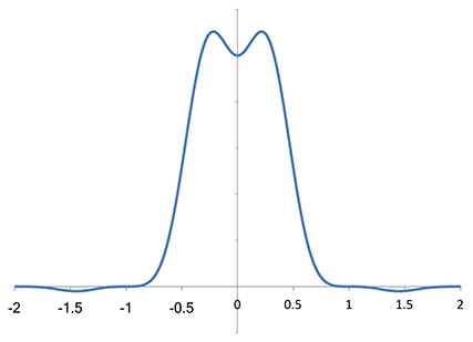
which in graphical form is now made up of five parabolas:
Graph of Magic Kernel Sharp (2013)
Compare this to the Lanczos-2 kernel:
Analytical formula for the Lanczos-2 kernel
which in graphical form is
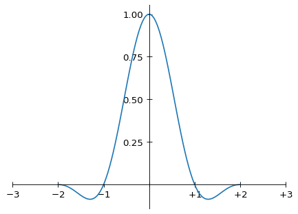
Graph of the Lanczos-2 kernel
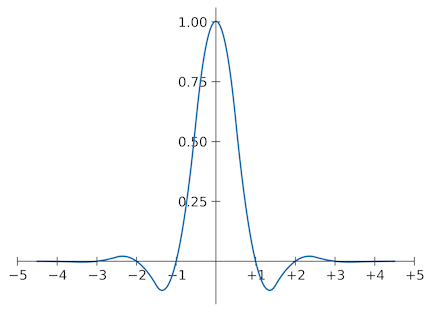
and the Fourier-ideal sinc function, which in graphical form, shown within this same domain, is
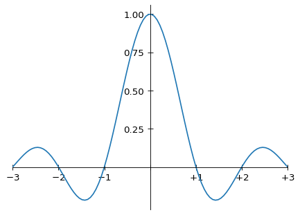
Graph of the ideal sinc function kernel, between −3 and +3
(and continues on outside this domain, of course, as it has infinite support). As noted above, the Magic Kernel Sharp 2013 kernel (I will drop the parentheses around “2013” from this point) has zeros at sampling positions x = ±1, as with the other two kernels shown here, but doesn’t have zeros at positions x = ±2. On the other hand, it has more weight in its negative lobes than Lanczos-2. Overall, however, the shapes of Magic Kernel Sharp 2013 and Lanczos-2 look quite similar.
To fully appreciate the antialiasing properties of the Magic Kernel Sharp 2013 kernel, however, I needed to move to Fourier space. I decided to perform the Fourier transforms numerically. For reference, and to check my code, I performed a numerical Fourier transform on the ideal sinc filter, with an arbitrarily-selected finite number of Fourier coefficients:
Numerical approximation of the Fourier transform of the sinc kernel
where we can see the Gibbs phenomenon (ringing) due to the finite number of coefficients chosen for this numerical example. The ideal sinc filter is unity inside the Nyquist domain or Brillouin zone (the Nyquist frequency is 1/2 in the units employed in this graph), and zero outside.
Analyzing the Lanczos-2 kernel in the same way, I obtained:
Fourier transform of the Lanczos-2 kernel, using the same numerical approximation
We can see that it starts to attenuate high-frequency components within the Nyquist domain; it continues to suppress frequencies outside that domain, and continues to drop until it crosses the axis. Note that it has a zero at twice the Nyquist frequency, i.e. the sampling frequency, which is f = ±1 in these units. This zero is important, because “foldover” will map the sampling frequency (and every multiple of it) to zero frequency under sampling (i.e. sampling places copies of the original spectrum at every integer), so a zero at f = ±1 means that nothing will end up at zero frequency from adjacent copies under sampling.
Numerically analyzing now the Fourier transform of the Magic Kernel Sharp 2013 kernel, I obtained:
Fourier transform of Magic Kernel Sharp 2013, using the same numerical approximation
It rises slightly before dropping toward zero, but otherwise has a fairly similar shape to the Lanczos-2 spectrum within the first Nyquist zone. But it appeared to me that Magic Kernel Sharp 2013 has a higher-order zero at f = ±1 (and f = ±2 as well). I zoomed the vertical axis to take a closer look:
Vertical zoom of the Fourier transform of Magic Kernel Sharp 2013
It is evident that the Magic Kernel Sharp 2013 kernel does indeed have high-order zeros (i.e. stationary points of inflection) at integer values of the sampling frequency. This explains why it has such good visual antialiasing properties: artifacts at low frequencies are particularly visually disturbing; these high-order zeros ensure that a substantial region of low-frequency space, after sampling aliasing, is largely clear of such artifacts, not just a small region around zero frequency.
When I zoomed the spectrum of the Lanczos-2 kernel to the same scale,
The same vertical zoom of the Fourier transform of the Lanczos-2 kernel
I made a rather startling observation: the Lanczos-2 kernel does not actually have a zero at integral multiples of the sampling frequency. Not only is the second zero at a frequency slightly higher than the sampling frequency (i.e., on the scale here, just below f = −1 and just above f = +1), but, more importantly, it is a first-order zero only (i.e. it “cuts through” the axis, approximately linear as it cuts through, rather than being a stationary point, let alone a stationary point of inflection, as we find for Magic Kernel Sharp 2013). Although this approximate zero for Lanczos-2 does a fairly decent job of suppressing foldover into the low-frequency domain overall, it is not comparable to the higher-order zero, at exactly the sampling frequency, of the Magic Kernel Sharp 2013 kernel—nor those possessed by Magic Kernel Sharp 2013 at multiples of the sampling frequency.
I noted in the introduction above that when Instagram engineer Georges Berenger came to me seeking to use Facebook’s resizing code for Instagram as well, he quickly proved that Instagram’s images were sharper than the ones that Magic Kernel Sharp 2013 was creating for Facebook. He asked me: could I fix this? He couldn’t deploy it to Instagram unless I could.
I looked back at my deployed 2013 code, and realized that if I simply hacked the “sharp” step into the form {−s, 4 + 2s, −s} / 4, I could change the value of s to provide any amount of extra sharpening desired—and it would be free. s = 0 corresponds to an identity kernel, i.e. no sharpening at all; s = 1 corresponds to the amount of sharpening required for Magic Kernel Sharp 2013 (actually, what Facebook actually uses is s = 0.9888, as I now admit above); s = 2 corresponds to twice as much sharpening; and so on.
We found that a value of s = 1.32 did the job required for Instagram.
Note that this “Magic Kernel Sharp+” is not intended to be a separate version of Magic Kernel Sharp that others should necessarily use. It is just a simple hack that allows the resized image to have more “pop” without any extra computational cost.
Well, a hack that powers all the photos on Instagram.
And it is this question of sharpness that led, six years later, to my next evolution of Magic Kernel Sharp.
We have seen above how the unique Fourier properties of the Magic Kernel Sharp 2013 kernel explain why its results are so remarkably free of aliasing artifacts, particularly at low frequencies. For most practical downsizing purposes, we can just apply it exactly as described above (and, indeed, it has been, on a rather large scale).
However, I did note above that in the limit k → 1, the kernel approaches {−1, 0, +34, 0, −1} / 32, which is a slight sharpening of the input image—and this sharpening can, indeed, be discerned in some images so transformed. (For regions with a reasonably constant second derivative, it contributes an additional 50% of the sharpening that the Sharp step should be providing.) The question naturally arises: could we refine the method by one more step, to try to remove this residual sharpening as much as possible, yielding something that is closer to an identity in the limit k → 1?
Indeed we can. Consider further convolving with the kernel {1, 0, 34, 0, 1} / 36, which by itself would be a slight blurring. The result is {−1, 0, 0, 0, 1154, 0, 0, 0, −1} / 1152. This is very close to an identity—and under the eight bits of dynamic range usually used for images, it is an identity.
In 2021 I therefore made the following ansatz: the 2021 version of the Magic Kernel Sharp kernel should include this extra convolution.
(Note: I did not deploy Magic Kernel Sharp 2021 to Facebook or Instagram. They continue to use Magic Kernel Sharp 2013 and Magic Kernel Sharp+ 2013 respectively. The 2021 improvement was personal hobby research only; I did not work on Photos at Facebook after 2015, although I did help Vjeux get pica JS to implement Magic Kernel Sharp in 2021, as Facebook wanted to use that JS library. Apologies if I have confused anyone in recent years on this point.)
So how should we view this refinement? Arguably, it is an improvement to the Sharp 2013 kernel itself. In 2013 I simply assumed a three-tap sharpening kernel {−1, +6, −1} / 4, without considering whether this is the ideal form for such a kernel. (Actually, the amount of sharpening was slightly different from this, as described above, but it’s close enough.) Our above considerations suggest that we should instead modify it to be the convolution of this with {1, 0, 34, 0, 1} / 36, namely, {−1, +6, −35, +204, −35, +6, −1} / 144.
In practice, then, the Magic Kernel Sharp method may be employed with either the simpler three-tap Sharp 2013 kernel {−1, +6, −1} / 4, yielding Magic Kernel Sharp 2013; or with the more spectrally flat Sharp 2021 kernel {−1, +6, −35, +204, −35, +6, −1} / 144, yielding Magic Kernel Sharp 2021, which does not blur or sharpen an image to at least nine bits of accuracy.
Graphically, Magic Kernel Sharp 2021 is the following kernel:
Graph of Magic Kernel Sharp 2021
Again, note that I now believe that most applications should use Magic Kernel Sharp 2013, unless there is a good reason to use Magic Kernel Sharp 2021.
As noted in the introduction above, in 2021 I analytically derived the Fourier transform of the Magic Kernel in closed form, and found, incredulously, that it is simply the cube of the sinc function. This implies that the Magic Kernel is just the rectangular window function convolved with itself twice—which, in retrospect, is completely obvious. (Mathematically: it is a cardinal B-spline.) This observation, together with a precise definition of the requirement of the Sharp kernel, allowed me to obtain an analytical expression for the exact Sharp kernel, and hence also for the exact Magic Kernel Sharp kernel, which I recognized is just the third in a sequence of fundamental resizing kernels. These findings allowed me to explicitly show why Magic Kernel Sharp is superior to any of the Lanczos kernels. It also allowed me to derive further members of this fundamental sequence of kernels, in particular the sixth member, which has the same computational efficiency as Lanczos-3, but has far superior properties. These findings are described in detail in the following paper:
In the research paper above I go into excruciating analytical detail as to why Magic Kernel Sharp is better than the Lanczos kernels, building on those Fourier spectrum observations above. But it’s easiest to cut to the chase and see for yourself with two telling examples.
The first example is an enlargement of a Gaussian blob:

Figure 35 of my paper showing that Magic Kernel Sharp does not have the pixelation problem of the Lanczos kernels
For enlarging, the flaws of the Lanczos kernels can lead to pixelation problems like these.
The second example is a reduction of a vertical grating:

Figure 37 of my paper showing that Magic Kernel Sharp does not have the beat problem of the Lanczos kernels
For reducing, these same flaws of the Lanczos kernels can lead to beat problems like these.
Note that the avoidance of these problems comes completely from the Magic Kernel part of Magic Kernel Sharp. It doesn’t matter whether you use the 2013 or 2021 version of Magic Kernel Sharp: neither of them has the fundamental flaws and artifacts inherent in the Lanczos kernels.
[2025 note: the easiest way to implement Magic Kernel Sharp is to look at Alain Viddeleer’s simple C/C++ implementation of it.]
After updating this page in February 2021 with Magic Kernel Sharp 2021, a question was repeatedly asked of me by authors of resizing libraries and applications: How do I implement it in practice? In November 2022 I apologized for burying the answer to that question in both the research paper above and the general ANSI C implementation below, and rectified this failure by adding the following.
In general, there are three ways that Magic Kernel Sharp 2021 can be implemented in practice:
For this reason, I supply here the explicit formula for the full Magic Kernel Sharp 2021 kernel for the “direct” implementation (3):
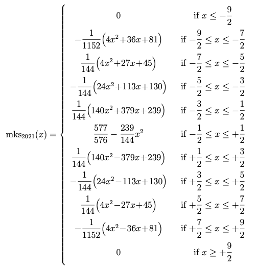
Analytical formula for Magic Kernel Sharp 2021
An alternative, equivalent formula for Magic Kernel Sharp 2021 that may be slightly more computationally efficient is

Alternative formula for Magic Kernel Sharp 2021
Likewise, an alternative, equivalent formula for Magic Kernel Sharp 2013 that may be slightly more computationally efficient is

Alternative formula for Magic Kernel Sharp 2013
(Hat tip to lakshayg for performing these simplifications when he implemented Magic Kernel Sharp in ImageMagick.)
I am happy to help anyone implementing Magic Kernel Sharp. Feel free to contact me directly.
So you have dropped the above formulas for the new Magic Kernel Sharp 2013 and 2021 hotness into your own image resizing library or application. How can you easily test that your implementation is correct?
In December 2024 I added two programs to my reference C implementation that makes this testing relatively simple.
First, you use one of those programs to create a “kernel test input” image. For Magic Kernel Sharp 2013 it is:
$ make_kernel_test_input 5 mks-2013-input.png
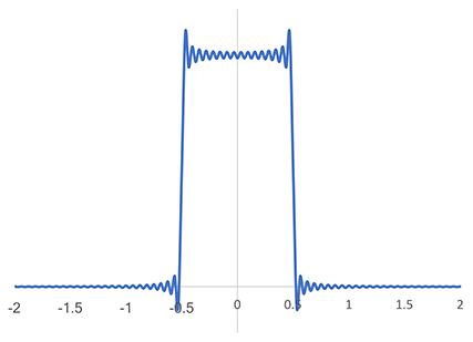
The first argument here, 5, is the “support” (total width for nonzero values) of the kernel, which for Magic Kernel Sharp 2013 is just 5, because it goes from −2.5 to +2.5. The second argument is just the filename of the image file you want it to create. Looking at that image file, mks-2013-input.png (you can download it from this link if you cannot build the programs yourself),

5 × 5 kernel test input file for Magic Kernel Sharp 2013
we see that it is a 5 × 5 image with a light gray one-pixel-wide vertical line centered on a dark gray background. (Use -h for a help screen, or -H for a horizontal rather than a vertical line.)
You now enlarge that image using your implementation of Magic Kernel Sharp 2013, by whatever suitably large factor you choose. For example, for my own reference implementation below, I can just do
$ resize_image mks-2013-input.png -k 100 -m MAGIC_KERNEL_SHARP_2013 mks-2013-jpc.png
to enlarge the test input image by a factor of 100 using Magic Kernel Sharp 2013. The result is mks-2013-jpc.png:

The result of my Magic Kernel 2013 implementation enlargement of the test input image
I now just run this through the second, analysis program:
$ analyze_kernel_test_output 5 100 mks-2013-jpc.png mks-2013-jpc.csv
where I needed to specify that the enlargement factor used was 100. The output file mks-2013-jpc.csv contains the program’s empirical computation of the kernel that the image resizing program has used. You can graph it using the application of your choice:

The empirically computed kernel for my implementation of Magic Kernel Sharp 2013
This agrees visually with what I showed above. Plotting the actual formula for Magic Kernel Sharp 2013 (above) in very thin orange over this empirical blue graph, you can confirm that the kernel has been correctly implemented (you may need to zoom your screen to see it):

The same blue graph, with the correct kernel overlaid in very thin orange
Similarly, to test, say, ImageMagick’s implementation of Magic Kernel Sharp 2013, we simply use it to do the enlargment:
$ magick mks-2013-input.png -colorspace RGB -filter MagicKernelSharp2013 -resize 10000% -colorspace sRGB mks-2013-magick.png

The result of ImageMagick’s Magic Kernel Sharp 2013 implementation enlargement of the test input image
We now run the second program to analyze this image:
$ analyze_kernel_test_output 5 100 mks-2013-magick.png mks-2013-magick.csv
Graphing the output, we see something similar to that above:

The empirically computed kernel for ImageMagick’s implementation of Magic Kernel Sharp 2013
One obvious difference is that the values are clearly quantized. Comparison with the correct kernel also shows slight deviations:

The same blue graph, with the correct kernel overlaid in very thin orange
I don’t believe that this is a serious problem, but I must admit that I don’t fully understand it. I expected that a high default internal quantum depth together with error diffusion dither being turned on by default would yield a result as good as my implementation. I will return to this below.
We can likewise test our implementations of Magic Kernel Sharp 2021 the same way. In this case the support is 9:
$ make_kernel_test_input 9 mks-2021-input.png
which generates the file mks-2021-input.png:

9 × 9 kernel test input file for Magic Kernel Sharp 2021
I can now enlarge this by a factor of 100 using my reference implementation via
$ resize_image mks-2021-input.png -k 100 -m MAGIC_KERNEL_SHARP_2021 mks-2021-jpc.png
which yields

The result of my Magic Kernel 2021 implementation enlargement of the test input image
$ analyze_kernel_test_output 9 100 mks-2021-jpc.png mks-2021-jpc.csv
Going straight to the comparison with the correct kernel in orange:

My implementation of Magic Kernel Sharp 2021 (blue) with the correct kernel overlaid in very thin orange
Again, my implementation appears to be correct.
Likewise, testing ImageMagick’s implementation of Magic Kernel Sharp 2021:
$ magick mks-2021-input.png -colorspace RGB -filter MagicKernelSharp2021 -resize 10000% -colorspace sRGB mks-2021-magick.png

The result of ImageMagick’s Magic Kernel Sharp 2021 implementation enlargement of the test input image
$ analyze_kernel_test_output 9 100 mks-2021-magick.png mks-2021-magick.csv
Again, going straight to the comparison with the correct kernel in orange:

ImageMagick’s implementation of Magic Kernel Sharp 2021 (blue) with the correct kernel overlaid in very thin orange
If you again zoom your screen so that you can see the orange curve, this result more unambiguously points to quantization as almost certainly the only root-cause of discrepancy. You can actually see the quantization in the enlarged image above—you can see vertical “strips”—which tends to confirm that I am mistaken in my understanding of either the high default quantum depth or the default use of error diffusion dithering in ImageMagick.
The reference implementation of Magic Kernel Sharp is contained in the following ANSI C *nix code:
There are twelve sample programs included:
There are also 82 executables of unit tests and death tests provided.
Instructions for building the code are contained in the _README file within the archive.
Note that all code provided here is from my personal codebase, and is supplied under the MIT-0 License.
I am happy to help anyone implementing Magic Kernel Sharp. Feel free to contact me directly.
If you like the Magic Kernel, then you may also find useful the following image processing resources that I have put into the public domain over the decades:
If you want to build a resizing engine from scratch, and want to use Magic Kernel Sharp 2013 for it, then this appendix is for you.
Let us denote by k the ratio of each dimension of the output image (in pixels) to that of the input image, so that k < 1 for a downsizing (reduction) and k >1 for an upsizing (enlargement). We don’t consider here the case where we might want to stretch the image in either direction, although different values of k for x and y can be trivially implemented in practice if needed. Indeed, for simplicity, let us just consider one dimension of the image; since the x and y kernels are manifestly separable, we simply need to repeat the resizing algorithm for each dimension in turn.
For downsizing, we are mapping many input pixels to one output pixel. Each output pixel location, say, i (integral), naively corresponds to the input pixel location y = i / k, which in general won’t be integral. For example, if we were reducing a 210-pixel-wide image down to a width of 21 pixels, then k = 1/10. Naively, we can visualize output pixel position 0 corresponding to input pixel position 0, output pixel position 1 corresponding to input pixel position 10, and so on, through to output pixel position 20 corresponding to input pixel position 200. (In practice, this description is true for the pixel tiles themselves, and we consider a given pixel’s “position” to be at the center of the pixel tile, so we actually have to apply half-pixel offsets to the input and output pixel positions: y + 1/2 = (i + 1/2) / k. However, for this example, let us ignore that bookkeeping subtlety, for simplicity, which merely determines the “starting point” of the pixel grid.)
For each such output pixel i, we overlay the Magic Kernel m(k y − i) onto the input image. E.g. for the middle output position i = 10 in our example downsizing, the kernel’s maximum occurs at y = i / k = 100, corresponding to x = 0 in the function m(x) above; it is zero for y < (i − 3/2) / k = 85, corresponding to x < −3/2 in the function m(x); and it is zero for y > (i + 3/2) / k = 115, corresponding to x > +3/2 in the function m(x).
At each integral position in y-space (the input image space) for which the kernel is nonzero, the unnormalized weight is set to the value of the kernel, i.e. m(k y − i). E.g. at y = 90 it is set to m(90/10 − 10) = m(−1) = 1/8.
We then sum all the unnormalized weights, and normalize them so that the resulting set sums to unity. This set of weights is then used to compute the intensity of that output pixel, as the weighted sum of the intensities of the given input pixels. (Note that, for a two-dimensional image, the set of weights for each output pixel in each dimension needs to only be computed once, and reused for all of the rows or columns in that stage of the resizing.)
After this downsizing with the Magic Kernel has been completed, the result is then convolved with the simple three-tap Sharp 2013 post-filter {−1/4, +3/2, −1/4} (in each direction) to produce the final Magic Kernel Sharp 2013 downsized image.
For upsizing, conceptually we still apply the Magic Kernel Sharp 2013 kernel, but the practical implementation looks somewhat different. In this case, each input corresponds to many output pixels. We therefore want to use the Magic Kernel as an “interpolation filter,” except that instead of just using the two nearest samples for the interpolation, as we usually do in mathematics, we will actually make use of three samples (because the support of the Magic Kernel is three units). For each output position, we map back to the input space, and center the Magic Kernel at that (in general non-integral) position. For each of the three input samples that lie within the support of that kernel, we read off the value of m(x) and use it as the unnormalized weight for the contribution of that input pixel to the given output pixel.
So what about the Sharp step? It is clear, from the above, that it must be applied in the same space that the Magic Kernel m(x) has been applied, because it is the convolution of the Magic Kernel and the Sharp 2013 kernel that is close to a delta function, and a convolution only makes sense when both functions are defined on the same space. In this case, that is the input space—not the output space, as it was for downsizing—because it is in the input space that we applied m(x). That implies that we must first apply the three-tap Sharp 2013 kernel, to the input image, before using the Magic Kernel to upsize the result. The combination of these two operations is the Magic Kernel Sharp 2013 upsizing algorithm.
Another very useful by-product of building the Magic Kernel arose when a number of teams within Facebook needed to create blurred versions of images—in some cases, very blurred.
I quickly realized that we could just use the Magic Kernel upsizing kernel as a blurring kernel—in this case, applied in the original image space, with the output image having the same dimensions as the input image. The amount of blur is easily controlled by specifying the factor k by which the Magic Kernel kernel is magnified in position space x, compared to its canonical form m(x) shown above; any value of k greater than 1 corresponds, roughly, to each input pixel being “blurred across” k output pixels, since we know that the standard deviation of the full continuous function m(x) is 1/2, so that the standard deviation of the sampled filter will be approximately k / 2, and hence a two-standard-deviation “width” will be approximately k pixels.
For k less than 1, we need to be a little more careful: k → 2/3 corresponds asymptotically to no blurring, since the support of the scaled Magic Kernel drops to less than the inter-pixel spacing for values of k < 2/3. To work around this, and still have a convenient “blur” parameter b that makes sense for all positive b, we can linearly interpolate between (b = 0, k = 2/3) and (b = 1, k = 1) for all 0 < b < 1, and then simply define k = b for b > 1. (With this definition, the two-standard-deviation “width” is still approximately equal to b, for all positive values of b.)
This “Magic Blur” algorithm allows everything from a tiny amount of blurring to a huge (and unlimited) blurring radius, with optimal quality and smoothness of the results. (More efficient ways of performing Gaussian blur have been noted; the Magic Blur was convenient in that it made use of existing hardware libraries and calling code stack.)
Magic Kernel Sharp can be used to resample data in any number of dimensions. I have implemented it for the three-dimensional case, using as an example one particular volumetric file format, in the code for the 3D generalization of the JPEG-Clear method.
In response to a question from Eddie Edwards, I looked into how Magic Kernel Sharp could be implemented for audio applications—or, really, any one-dimensional signal processing application. The C code provided above, which includes a Kernel class, is optimized for multi-dimensional applications, where the size of each dimension is relatively “small” (in the thousands), but where the multiple dimensions (typically two or three) means that it is worth precomputing the kernels for every output position of each dimension, as they are then applied many times for each value of the hyperplanes orthogonal to that dimension.
This approach is not suitable for one-dimensional applications like audio. Here the kernel will be applied once only for each output position, unless the resizing factor happens to be a simple enough rational number that the kernel repeats in a useful way. The size of the input is likewise relatively unlimited, and indeed there will be streaming applications where the input signal will be streamed through fixed kernels, rather than kernels moving along a fixed pre-loaded signal.
At that point in time I didn’t have a good, general purpose implementation of Magic Kernel Sharp for such one-dimensional applications. However, to answer Eddie’s specific question—could it be used to convert between 48kHz and 96kHz audio?—I coded that up as a special case.
Since that time, I have implemented a general-purpose sampling program that can resample to any arbitrary sample rate.
The following code only works on 16-bit PCM WAV files, simply because that was the simplest format wrapper for me to implement, but the code is completely general and could easily be dropped into any proper audio processing system:
There are two sample programs included:
There are also 66 executables of unit tests and death tests provided.
Instructions for building the code are contained in the _README file within the archive.
Note that all code provided here is from my personal codebase, and is supplied under the MIT-0 License.
The programs both use Magic Kernel Sharp 6 with the v = 7 approximation to the Sharp kernel (i.e. the best version of Magic Kernel Sharp computed in my paper above), so that the Sharp kernel always has 15 taps.
For the halving and doubling program, the Magic Kernel has 12 taps for halving, and two alternating sets of 6-tap kernels for doubling. This means that, if employed in a streaming context, it would have an unremovable latency of 203 microseconds, due to the trailing tails of the two kernels.
The general program extends this “repeating kernel” methodology to any resampling factor that is rational (which is, in practice, generally the case).
For general downsampling, a potential new issue arises, discussed in the Facebook post thread above: the Magic Kernel Sharp kernel does not have vertical walls, but rather has a finite “roll-off.” If the input audio has appreciable signal around the new Nyquist frequency, then the portion of it just above the new Nyquist frequency will not be fully filtered out before the resampling, and will be aliased to just below the new Nyquist frequency. Whether this is important or not depends on the application; in Eddie’s case, the input signal was always effectively low-pass filtered to audio range, and the resampling rates were always 44.1 kHz or more, so that this was not an issue.
In image applications, this aliasing generally does not lead to appreciable visual artifacts, because the resulting aliased signal is itself close to the Nyquist frequency, and visually tends to average out. For audio, on the other hand, frequency can be discerned directly by your ear, and such aliasing may be detrimental, depending on the content and context.
Thus the general resampling program includes an optional command-line switch that effectively halves the bandwidth of the Magic Kernel Sharp filter. This puts the first sixth-order zero at the new Nyquist frequency, while retaining those high-order zeros at multiples of the sampling frequency. This will do a good job of masking off any significant spectral energy at the new Nyquist frequency. Note, however, that any significant energy between the Nyquist and sampling frequencies may still be aliased. This method is also about seven times slower than the standard method, because the normal factorization of Magic Kernel Sharp into the Magic Kernel and Sharp steps no longer applies, and the full (wider) Magic Kernel Sharp kernel must be applied in the larger sample space.
The programs seem to work pretty well. However, even though I said in the research paper above that Magic Kernel Sharp 6 might fulfill high-precision needs, analyzing a one-dimensional case like this is already convincing me that higher generations might be desirable for some applications. That’s not too difficult to do, but I haven’t done it at this time. Moreover, the eight bits of accuracy targeted in the paper for the Sharp kernels looks inadequate for audio that is typically 16 to 24 bits—although it is worth keeping in mind my observation that the Sharp kernel simply flattens the frequency response within the first Nyquist zone, with the antialiasing properties all being contained in the Magic Kernel (where higher generations mean more decibels of suppression). And either of these improvements would, of course, increase the unremovable latency: for example, for the halving and doubling use case, every extra generation of the Magic Kernel would add 10 microseconds, and every extra approximation to the Sharp filter would add 21 microseconds.
As noted above, Magic Kernel Sharp downsizing (either the 2013 or the 2021 version) can be implemented even using hardware-assisted libraries that only provide same-size filtering and non-antialiased downsizing, as was the case for my 2013 implementation of it at Facebook:
First, scale up the Magic Kernel by the factor 1 / k as described above, but apply it as a regular filter to the input image. (This blurs the original image in its original space, but it will not be blurred in the final output space, after downsizing).
Next, apply the best downsizing method available in the hardware-assisted library (say, bilinear). This downsizing may not be properly antialiased for general images, but it suffices for the image that has been pre-blurred by the Magic Kernel.
Finally, apply the Sharp filter (either the 2013 or the 2021 version) to the downsized results.
The results are for most practical purposes indistinguishable from those obtained from the full Magic Kernel Sharp algorithm, and are immensely better than using a hardware-assisted downsampling algorithm that is not properly antialiased.
This might seem like a strange question, since I started in 2006 with the doubling of an image, with the original “magic” kernel. Why do we care about that now?
In practical terms, I care because the halving and doubling kernels are used in my Magic Edge Detector, my mipmapping encoding, and its three-dimensional generalization. But even beyond this, in terms of theoretical rigor, it is worth “closing the loop” to see how the kernel that started all of this off in 2006 is transformed into its final form.
The answer to this question, though, is actually far from obvious. Could it be that we should just apply the Sharp 2013 or 2021 kernel to the output of the original “magic” kernel?
It’s straightforward to see that this would not yield an ideal result. In the above, we have never applied the Sharp kernel to anything but the output of the (generalized) Magic Kernel; this is what all of our analysis tells us is the optimal convolution of kernels. And it is easy to verify that the Magic Kernel for k = 2 or k = 1/2 is not exactly equal to the original “magic” kernel.
For example, for the doubling Magic Kernel, where the “tiled” positions of interest are {−5/4, −3/4, −1/4, +1/4, +3/4, +5/4}, we find that the weights are {1, 9, 22, 22, 9, 1} / 32. This is subtly different from the {1, 3, 3, 1} / 4 = {0, 8, 24, 24, 8, 0} / 32 of the original “magic” kernel. The difference may not seem to be great—we have just taken 1/32 from each of the four outer weights and donated it all to the two central weights—but such an apparently small change in position space has a disproportionately large impact on those high-order zeros in Fourier space, which give Magic Kernel Sharp (either in its 2013 or its 2021 incarnation) its most magical properties.
(Indeed, if you have read my research paper, it will be clear to you that the original “magic” kernel is actually just the linear interpolation kernel, i.e. “Magic Kernel 2,” for the special values of k = 2 and k = 1/2. It is only if you repeatedly resize an image with that original “magic” kernel that the result approaches that of the Magic Kernel.)
Thus, in general, we should simply use the full Magic Kernel Sharp algorithm (either its 2013 or its 2021 version) with k = 2 or k = 1/2 to define the “doubling” and “halving” kernels.
Let me note here a subtle issue that arises when one wants to numerically analyze the mathematical properties of Magic Kernel Sharp, as we have done above: edge effects.
Mathematically, when one defines a kernel, it is overwhelmingly convenient to only consider those that are translation-invariant—the kernel is the same shape no matter where it is applied, i.e. k(x, y) = k(x − y)—which means that its application to a given signal is simply the convolution of that (translation-invariant) kernel function k(x) with the signal s(x), and of course the Fourier transform of a convolution of functions is simply the product of the Fourier transforms of the functions. Such a simplification is implied in all of the above Fourier analyses.
It might seem that all of the kernels considered above are translation-invariant; and, as presented, indeed they are. The problem arises when we consider a sampling grid of finite extent, as we have in practice for images. Translation-invariance for the purposes of convolution and Fourier analysis requires that we assume “periodic boundary conditions” in position space, i.e. that the position “to the left” of the leftmost pixel is actually the rightmost pixel. This works really well for mathematical Fourier analysis (and theoretical physics): all the assumptions and properties continue to work perfectly. But it’s just not an option for image processing: you can’t have the left edge of an image bleeding over and appearing on the right edge!
In reality, what we do in image processing when the mathematics tells us to “go to the left of the leftmost pixel” is to just stay on the leftmost pixel. We don’t “wrap around” to the rightmost pixel; we just “pile on” on that leftmost one. Any theoretically-specified pixel locations to the left of the image are replaced by that leftmost pixel, and likewise for the other three sides.
One might think that this “piling on” might lead to weird visual artifacts, but, in fact, in almost all (i.e., “nonpathological”) situations, it doesn’t. All that we are doing, effectively, for the purposes of any filtering, is “extending” the image into the surrounding empty space, simply copying the pixel value of the closest edge or corner pixel that is within the image. We then apply the filter, and then trim off these extended edges. We can call this “extension boundary conditions.”
Visually, extension boundary conditions work great; it is as good as it can possibly get. Mathematically, it makes everything a mess.
A useful working paradigm for numerical analysis of the above kernels is therefore as follows: write the code so that there is a flag that specifies whether the kernel should use periodic boundary conditions or extension boundary conditions. Use the periodic boundary conditions option when analyzing mathematical properties (Fourier properties, composition of kernels, etc.). Use the extension boundary conditions option for all practical applications to images.
This does also mean that there can be very slight differences in how the Magic Kernel Sharp kernel is implemented in practice, depending on whether it is defined in terms of two kernel applications (Magic Kernel and then Sharp), or as a single kernel application (the composition of Magic Kernel and Sharp). With periodic boundary conditions, the two implementations should be identical (but see below), and the choice comes down to convenience. For extension boundary conditions, however, edge effects for each kernel application mean that the two operations are not identical. Visually, of course, these differences in edge effects should be completely negligible. They only need to be kept in mind if one is trying to, for example, build unit tests to confirm the correctness of the kernels as implemented in code, as I have done for the reference implementation provided below.
A further complication arises if, in composing the two kernels, each of the two are normalized before being composed, and then the composed result is again normalized. (This can easily occur if the kernel-building class automatically normalizes each kernel that it constructs.) Except for special values of k, the normalization of the raw weights for the Magic Kernel will not always be exactly the same for every output position, and the normalization step fixes that. However, normalization and composition do not commute, so that normalizing and then composing with the Sharp kernel will yield a very slightly different result than if the unnormalized kernel was composed with the Sharp step and only then was normalized afterwards. Again, the effects are negligible in practical terms, but do impact what unit tests can be constructed.
This page describes personal hobby research that I have undertaken since 2006. All opinions expressed herein are mine alone. I put the Magic Kernel into the public domain, via this page and its predecessor on my previous domain, in early 2011, and it has also been pointed out that both it and the subsequent sharpening step are both encompassed within the general theory of cardinal B-splines, explicitly confirming that Magic Kernel Sharp was contained within prior art and hence not subject to any patents. All code provided here is from my personal codebase, and is supplied under the MIT-0 License.
© 2006–2026 John Costella