JPEG-Clear is a progressive image (mipmapping) algorithm: a method for storing and transmitting successive approximations to a JPEG or PNG image through a low-bandwidth channel using nothing more than standard JPEG and PNG files. The initial approximation files are very small, allowing a quick rendering of the overall gist of the image; the use of Magic Kernel Sharp for these renderings yields optimal-quality, smooth and unaliased approximations. Successive files provide more and more detail, again using the optimal Magic Kernel Sharp rendering engine.
For a JPEG image, the total set of files typically has around the same size as the original JPEG file; in other words, the method rearranges the image data into a “top-down” collection of files.
A reference ANSI C implementation of JPEG-Clear is provided at the bottom of this page.
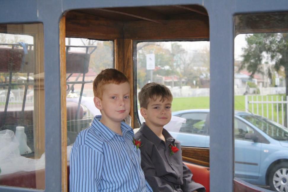
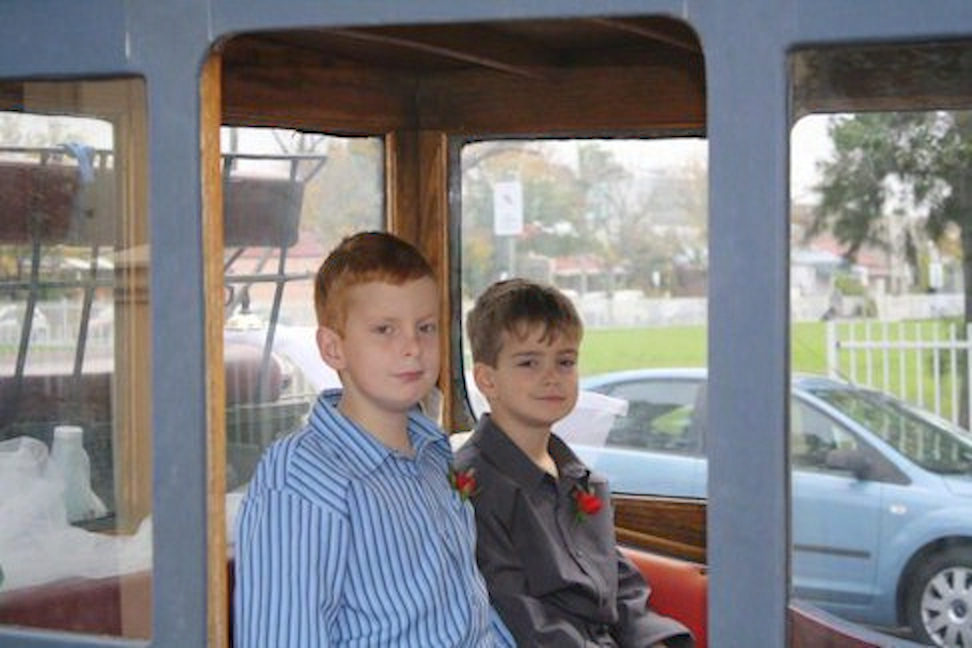
For simplicity, imagine we wanted to view a web page containing the following image:
mattjack.jpg (972 x 648 pixels, 77 KB):
Let us pretend, for the point of illustration, that the channel through which this image is being transmitted is extremely low bandwidth (by today’s standards)—say, 1 KB/s. This 77 KB image would then take 77 seconds to be fully transmitted. (Yes, this was our life in the mid-1990s.)
Using JPEG-Clear, the following image would appear after just two-thirds of a second:

Initial image that would appear using JPEG-Clear
The result is blurry, but is not a bad effort, given that it is based on only about 700 bytes of data.
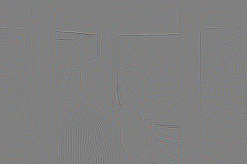
After another second or so, JPEG-Clear replaces the image with this:
Second image that would appear using JPEG-Clear
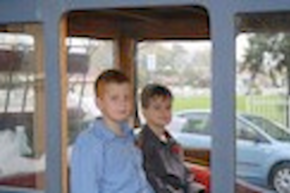
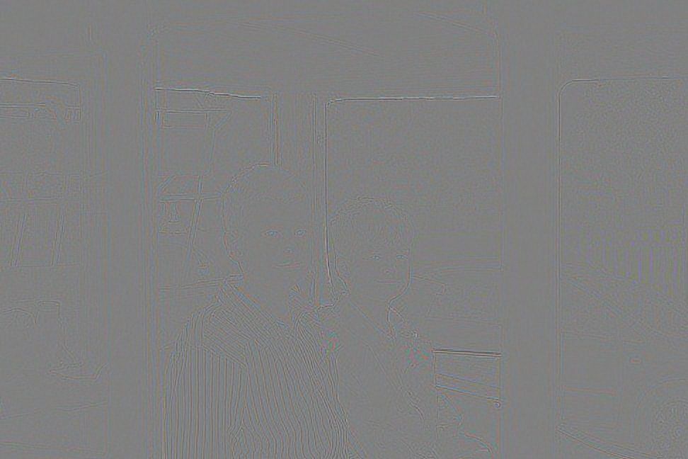
and, after another two seconds, with
Third image that would appear using JPEG-Clear
Even with this painfully slow connection, someone browsing this page would have a good idea of what the image showed within seconds, without having to wait over a minute for the entire image file to “crawl down the page.”
This example is contrived; but think of the original ten-megapixel photograph that this image was derived from. There is no need to store different versions of the image at different resolutions: it can be downloaded progressively, “top-down,” and rendered at any desired size.
For completeness, I show what would be rendered after another four seconds:
Fourth image that would appear using JPEG-Clear
After ten more seconds:

Fifth image that would appear using JPEG-Clear
And after 25 more seconds:
Sixth image that would appear using JPEG-Clear
Finally, after another minute, something effectively equivalent to the original image at full detail would be shown:
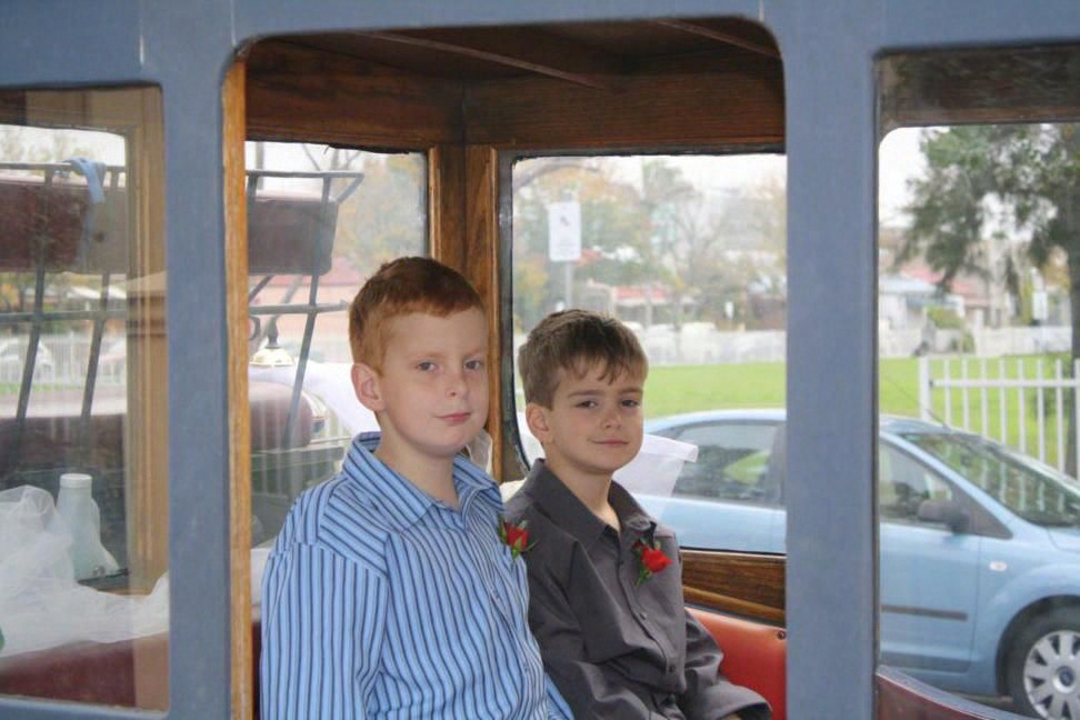
Final image that would appear using JPEG-Clear
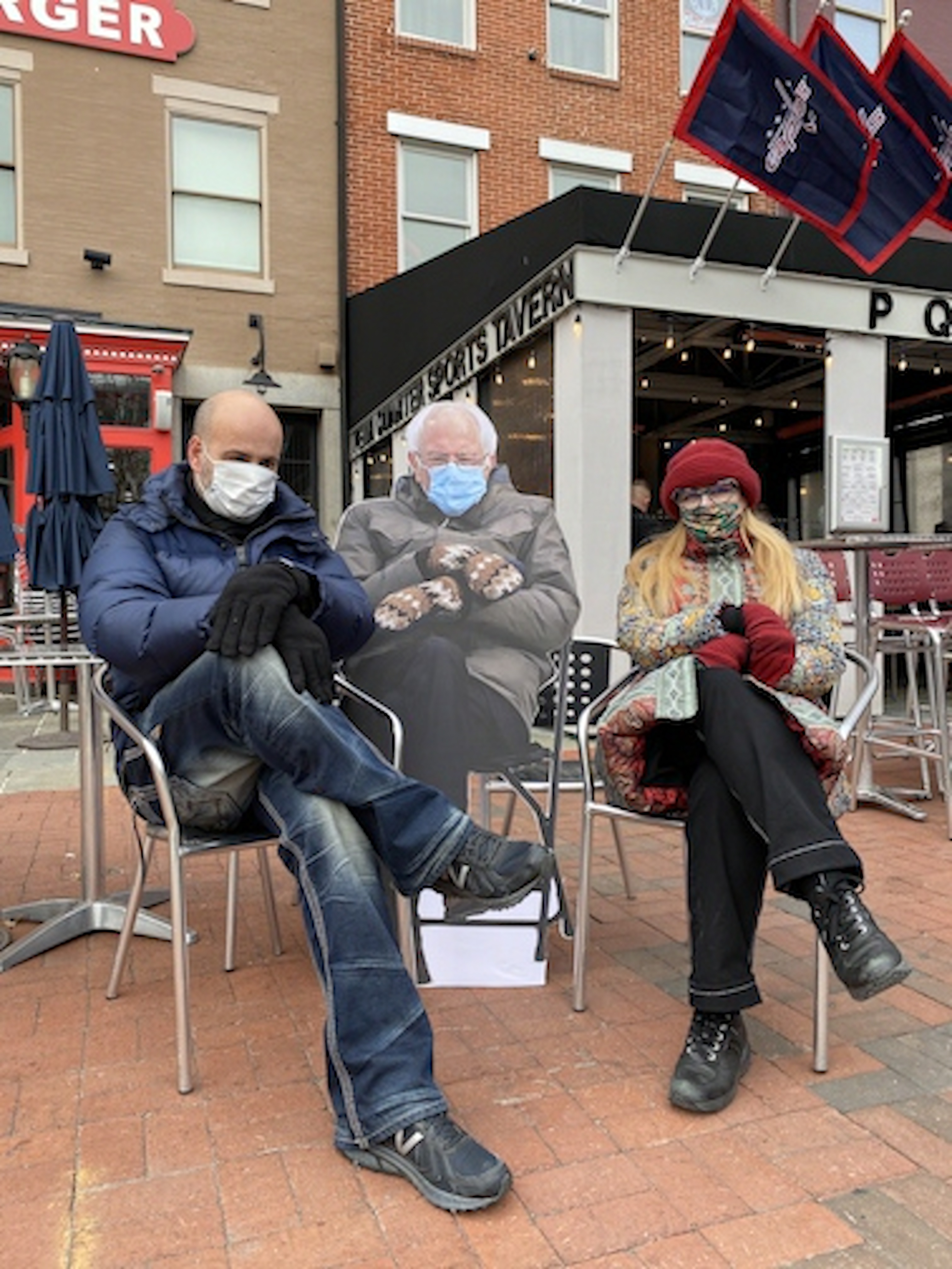
As a more modern example, consider the following 3024 x 4032 iPhone 12 Pro photo, saved with JPEG quality 95:
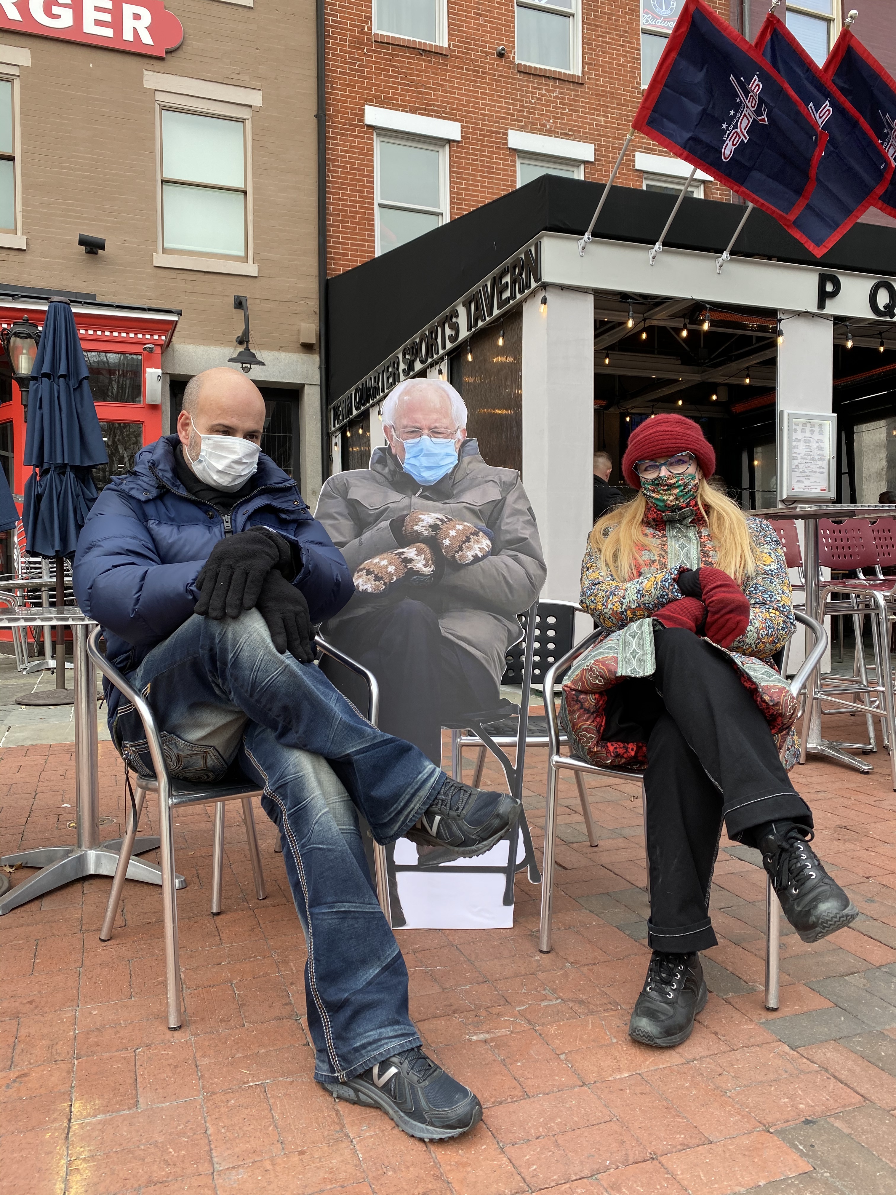
bernie.jpg (3024 x 4032 pixels, 4126 KB)
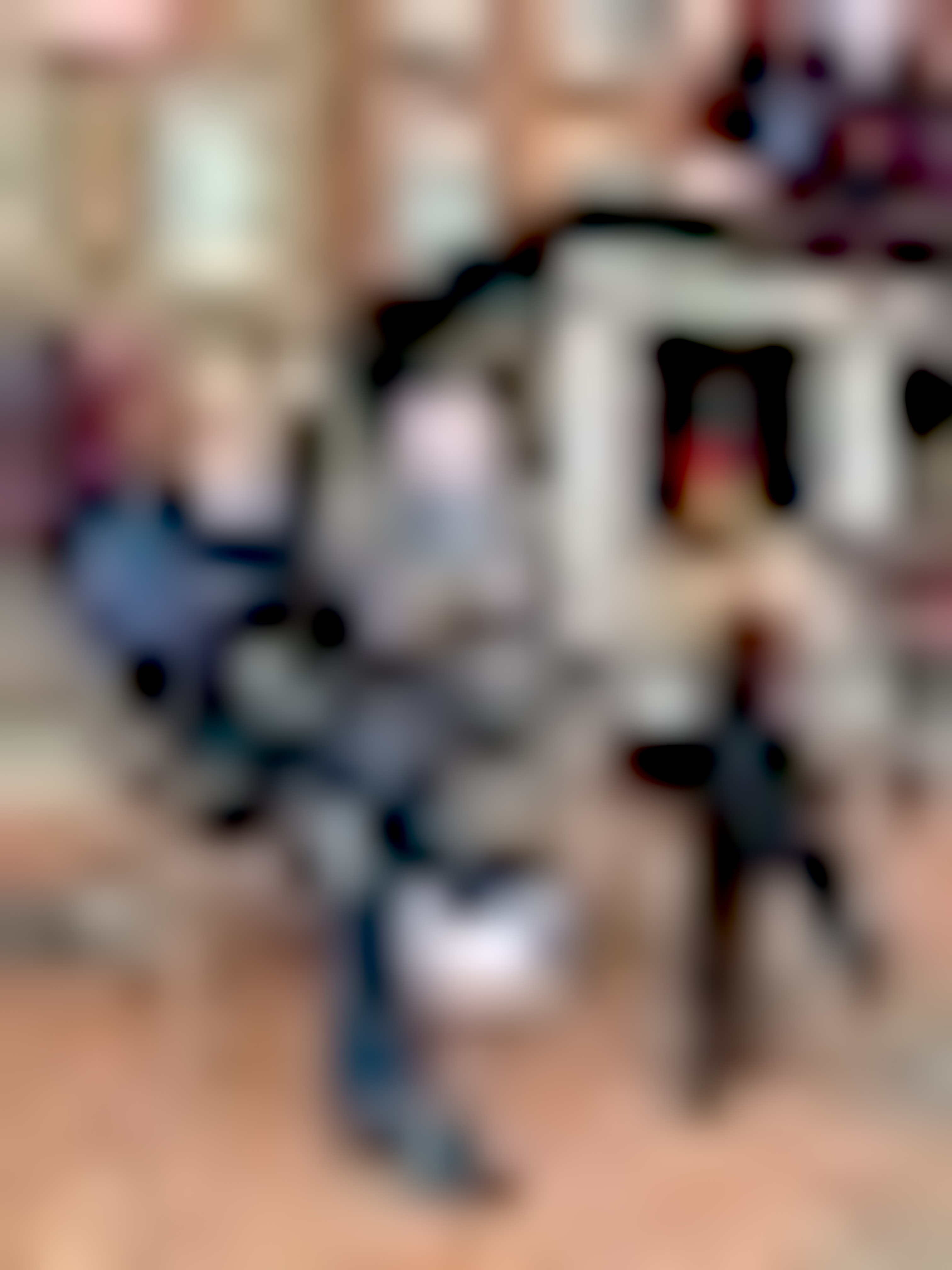
After around 800 bytes of data has been downloaded, the following approximation would be shown:
First image that would appear using JPEG-Clear
After another 1.5 KB:
Second image that would appear using JPEG-Clear
After another 3.8 KB:

Third image that would appear using JPEG-Clear
After another 10 KB:

Fourth image that would appear using JPEG-Clear
After another 30 KB:

Fifth image that would appear using JPEG-Clear
After another 107 KB:
Sixth image that would appear using JPEG-Clear
After another 332 KB:

Seventh image that would appear using JPEG-Clear
After another 1.2 MB:

Eighth image that would appear using JPEG-Clear
Finally, after another 3.2 MB, something effectively equivalent to the original image above would be shown:

Final image that would appear using JPEG-Clear
The total amount of image data downloaded for the complete set is about 4.8 MB, which is slightly more than the original 4.1 MB JPEG file. But note that three-quarters of this total comes from the final approximation; If this slight increase in overall storage is an issue, JPEG-Clear allows the JPEG compression to be set for each approximation.
Let’s go back to the original image above:
mattjack.jpg (972 x 648 pixels, 77 KB):
The JPEG-Clear algorithm starts by storing some metadata about the image—whether it is PNG, its dimensions, and the version and approximation of Magic Kernel Sharp that will be used—in a 2x1-pixel PNG image file, mattjack.jpg.jpc.x.png, 74 bytes in size, which will be the first file downloaded. The filename looks complicated, but its structure allows easy downloading of JPEG-Clear file sets, simply as a set of standard PNG and JPEG images. It is best understood by building up the extensions:
mattjack.jpg The original image filename
mattjack.jpg.jpc Identifies a JPEG-Clear file set
mattjack.jpg.jpc.x The metadata file is indexed as
“x”; other indexes will be described below
mattjack.jpg.jpc.x.png Saved as a standard PNG image
Why store this metadata in a PNG file rather than a plain binary file? Because most network systems will not allow arbitrary binary files to be transmitted; keeping this data in the same sort of file type (image file) as the others in the JPEG-Clear file set avoids this issue.
JPEG-Clear next creates a small thumbnail of the image, reduced in size using the gold standard Magic Kernel Sharp method, by a factor that is the power of two (here 64) that is sufficient to make each dimension of the thumbnail no greater than 16 pixels:
![]()
mattjack.jpg.jpc.a.png (16 x 11 pixels, 651 bytes)
The index “a” here identifies the “base” image file in the JPEG-Clear file set. For the command-line programs, it is referred to as “scale 4,” because each of the dimensions can be represented with just 4 bits (since a dimension can never be zero; they are always rounded up). It is actually much more efficient to store this tiny base file in the exact (lossless) PNG file format, rather than try to use JPEG compression on it.
Now, the first approximation shown earlier is obtained by simply downloading these two files—the metadata file “x” and the base image file “a”—and upsizing, using Magic Kernel Sharp, this thumbnail by a factor of 64 back up to the original size and dimensions:
The image mattjack.jpg.jpc.a.png above upsized by a factor of 64 using Magic Kernel Sharp
To obtain the next approximation of the image, JPEG-Clear upsizes the “a” thumbnail by a factor of 2, again using Magic Kernel Sharp. It then compares this to the exact image obtained by downsizing the original image by a factor of 32. The difference between the two, by channel and pixel, is encoded into a new image, using a nonlinear transformation that maps differences (between −255 and +255) to the values than be represented by bytes (0 through 255) in such a way that small differences are encoded losslessly, but larger differences are quantized, with the quantization error being −1, 0, +1, or +2. This difference-encoded image is then written out with JPEG compression (with a quality factor slightly less than 100) as mattjack.jpg.jpc.b.jpg:
![]()
mattjack.jpg.jpc.b.jpg (31 x 21 pixels, 1.2 KB)
A receiving application would reconstruct the best available approximation to the original image at scale 5 from the two files mattjack.jpg.jpc.a.png and mattjack.jpg.jpc.b.png, and then upsize it by a factor of 32 to yield the second approximation shown above:
The result of reconstructing mattjack.jpg.jpc.a.png with mattjack.jpg.jpc.b.jpg and then upsizing by a factor of 32
Note that this reconstruction is an approximation for two reasons: because the differences may, in general, be quantized; and because the “diff” file is compressed using JPEG compression.
The process continues up through the scales, with each preceding approximation being subtracted from the exact image at each scale, and the diff being written out in this encoded form:
![]()
mattjack.jpg.jpc.c.jpg (61 x 41 pixels, 2.0 KB)
mattjack.jpg.jpc.d.jpg (122 x 81 pixels, 4.4 KB)
mattjack.jpg.jpc.e.jpg (243 x 162 pixels, 11 KB)
mattjack.jpg.jpc.f.jpg (486 x 324 pixels, 26 KB)
mattjack.jpg.jpc.g.jpg (972 x 648 pixels, 59 KB)
Absolutely. Any video stream could be broken into a “base” video stream, plus “diff” video streams, in exactly the same fashion as shown above for still images.
A playback application need only subscribe to the “diff” streams necessary for rendering at the desired resolution. Alternatively, over an unreliable bandwidth connection (such as the Internet), a playback application can “drop” its subscription to higher-detail diff streams when bandwidth degrades, and “resubscribe” to them if and when bandwidth improves again.
Although not its primary goal, JPEG-Clear can handle images stored losslessly, providing efficient JPEG-based approximations but ultimately supplying the complete exact original image, with an important caveat: the same JPEG library must be used for encoding and decoding. The reason is that a given JPEG file can be interpreted slightly differently by different libraries, and in general it is impossible to correct for these differences ahead of time.
With that caveat, it is straightforward to understand how JPEG-Clear can provide the final exact, lossless image from the set of approximations. To do this, it stores an extra two “diffs” which, when combined with the JPEG approximations, allow the original image to be reconstituted losslessly.
For example, imagine that we started with the following lossless image:

sally.png (214 x 320 pixels, 115 KB)
The JPEG-Clear library converts this to the following file set:
![]()
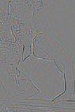
sally.png.jpc.a.png (7 x 10 pixels, 331 bytes)
![]()
sally.png.jpc.b.jpg (14 x 20 pixels, 922 bytes)
![]()
sally.png.jpc.c.jpg (27 x 40 pixels, 1.2 KB)

sally.png.jpc.d.jpg (54 x 80 pixels, 2.0 KB)
sally.png.jpc.e.jpg (107 x 160 pixels, 4.2 KB)
sally.png.jpc.f.jpg (214 x 320 pixels, 8.9 KB)
sally.png.jpc.y.png (214 x 320 pixels, 102 KB)

sally.png.jpc.z.png (214 x 320 pixels, 1.0 KB)
The first six files are exactly what would have been produced if the original image had been JPEG. The last two files, on the other hand, are again stored in the lossless PNG format, and encode the difference between the original image and the approximation obtained by combining the first six files. Using all eight files together, JPEG-Clear can reconstitute sally.png, exactly.
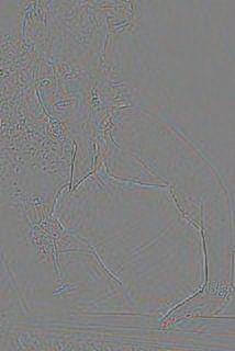
It may seem strange that sally.png.jpc.y.png is by far the largest of the six files by size, but appears to contain far less information that its predecessors. The reason is that the differences it is encoding are small, but necessary if one wishes to have absolutely lossless compression. Amplifying the intensity scale referenced to mid-gray shows what it is storing:
The image sally.png.jpc.y.png with intensities amplified around mid-gray
In other words, it is simply supplying the “JPEG noise”, not discernable to the naked eye, but necessary for a lossless reconstruction.
The final image file, sally.png.jpc.z.png, is needed because, as described above, the nonlinear encoding of deltas leads to quantization of large deltas—including those encoded in sally.png.jpc.y.png itself. In this particular case, none of those deltas were in fact quantized, so that sally.png.jpc.z.png is pure mid-gray, but in general this final diff file is necessary for ensuring an absolutely lossless reconstruction of the original image.
It may seem, from this example, that the JPEG-Clear transformation allows a slight extra compression of lossless images: the original PNG file was 115.3 KB in size, whereas the eight JPEG-Clear files total only 114.8 KB (and there are examples where this delta is greater). However, this is only true in this particular contrived example because the original image was a continuous-tone photograph—for which lossless compression is rarely, if ever, used (except, perhaps, for medical imaging purposes, where a lossless reconstruction of the original image may be needed on legal grounds). Consider, as a contrary example, the following screenshot:

bing.png (717 x 395 pixels, 83 KB)
The JPEG-Clear file set corresponding to this lossless PNG image consists of the following:
![]()
bing.png.jpc.a.png (12 x 7 pixels, 314 bytes)
![]()
bing.png.jpc.b.jpg (23 x 13 pixels, 895 bytes)
![]()
bing.png.jpc.c.jpg (45 x 25 pixels, 1.2 KB)

bing.png.jpc.d.jpg (90 x 50 pixels, 2.4 KB)

bing.png.jpc.e.jpg (180 x 99 pixels, 5.3 KB)

bing.png.jpc.f.jpg (359 x 198 pixels, 14 KB)
bing.png.jpc.g.jpg (717 x 395 pixels, 41 KB)
bing.png.jpc.y.png (717 x 395 pixels, 386 KB)

bing.png.jpc.z.png (717 x 395 pixels, 9.5 KB)
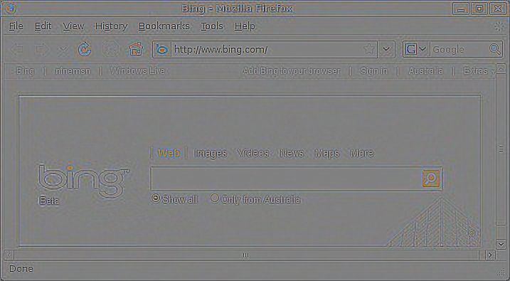
In this case, the main “lossless diff,” bing.png.jpc.y.png, is more than four times larger than the original file! The reason is that a screendump like this typically consists of large areas of constant intensity plus sharp edges (in both luminance and chrominance), for which a JPEG approximation provides a poor representation (from a lossless point of view): encoding the differences from the approximation—including the JPEG noise caused by those sharp edges—is much more costly than encoding the original image. This is not to say that the JPEG appproximation is poor, from a visual perspective: the full-scale approximation (i.e. without using the “y” and “z” PNG diff files) is this:

Full-scale lossy JPEG-Clear approximation of bing.png
It would also be possible to implement the JPEG-Clear algorithm using lossless image storage throughout. However, each “diff” image would need one extra bit of information, to encode the sign of the difference. This would be feasible in custom imaging fields such as medical imaging, but is not feasible for general-purpose use.
Yes: see here.
The reference implementation of JPEG-Clear is contained in the following ANSI C code:
There are two sample programs included:
There are also 79 executables of unit tests and death tests provided.
Instructions for building the code are contained in the _README file within the archive.
Note that all code provided here is from my personal codebase, and is supplied under the MIT License.
If you like JPEG-Clear, then you may also find useful the following image processing resources that I have put into the public domain over the decades:
© 2006–2026 John Costella