You can learn how Bear works by reading or working through this simple tutorial.
You have two options:
All the commands I use below are listed here.
If you have built Bear and added it to your path, then execute this command:
$ memory_bear
You should see output that looks something like this (details of all screenshots may vary):
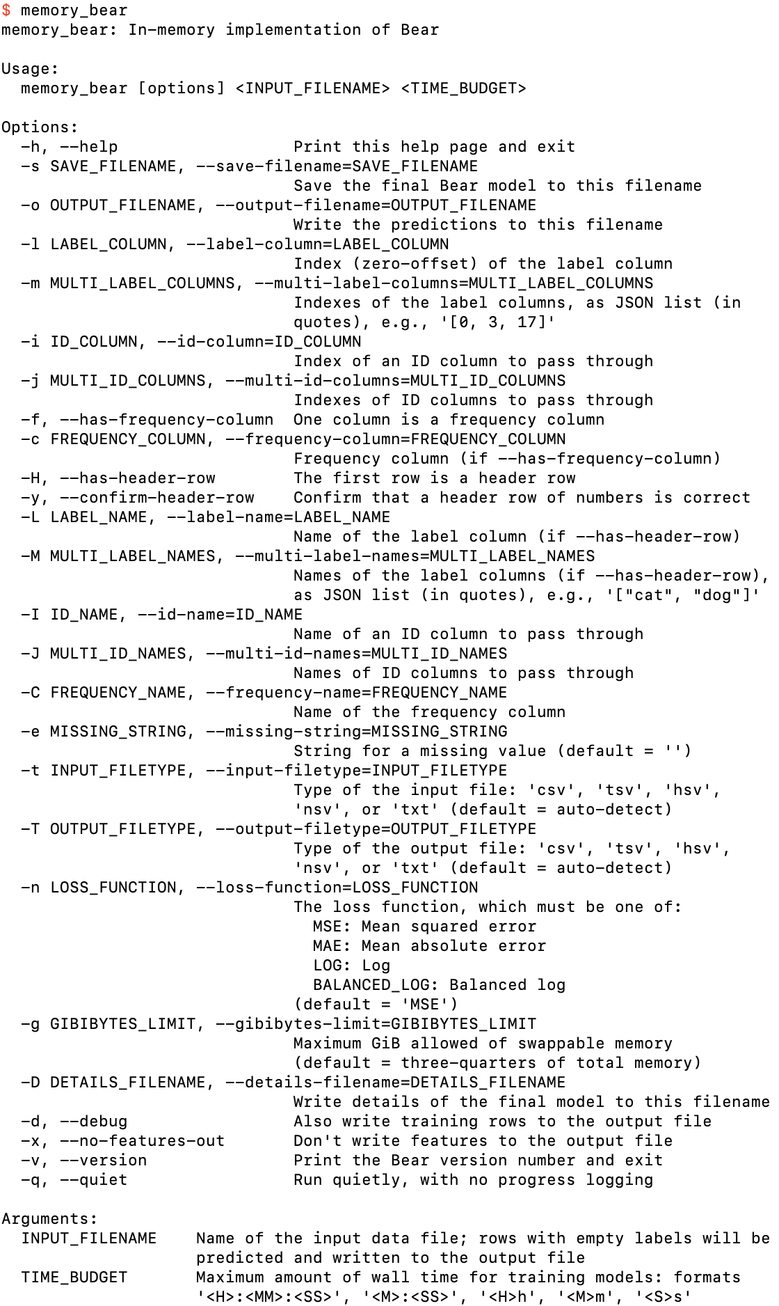
The help screen that you should get from memory_bear if you run it with no arguments
You can see from the “Arguments:” section at the bottom of this screenshot that memory_bear has two mandatory arguments: INPUT_FILENAME and TIME_BUDGET. Let’s just create an empty input file,
$ touch empty.csv
and run memory_bear on it, specifying a time budget of, say, one minute:

Running Bear with only the mandatory arguments
Okay, so we learn that it’s mandatory to specify the label column(s) using one of these four options. Let’s just specify it as column 0:

After specifying a label column
So we also need to specify a filename for saving the Bear model or writing an output file with predictions (or both). Let’s just specify a Bear model filename:
After specifying a model save filename as well
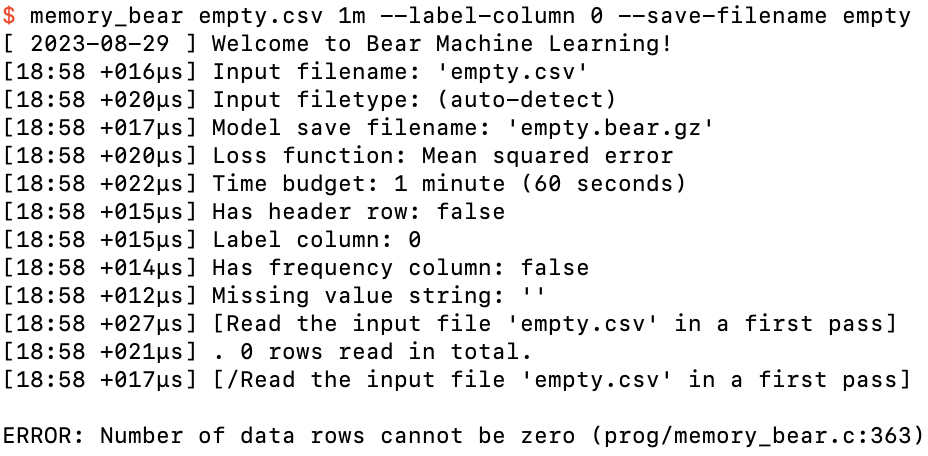
Now we’re getting somewhere! Bear fired up with a welcome message, and then some feedback to us of its parsing of what we have asked of it. At the left side of each log line you will always see the local time (to the minute) and the time that has elapsed since the last log line. (The first log line tells you the local date when execution started.)
We can see that Bear did a first pass over the input file, but then it told us that an empty data file isn’t allowed!
So let’s create the simplest possible dataset: a single example (row), with no features, and just a label value, in single-label.csv:
File with just a single label value
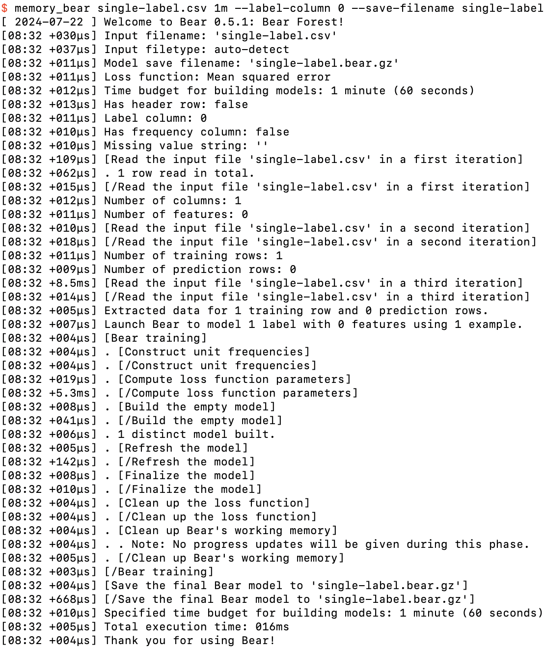
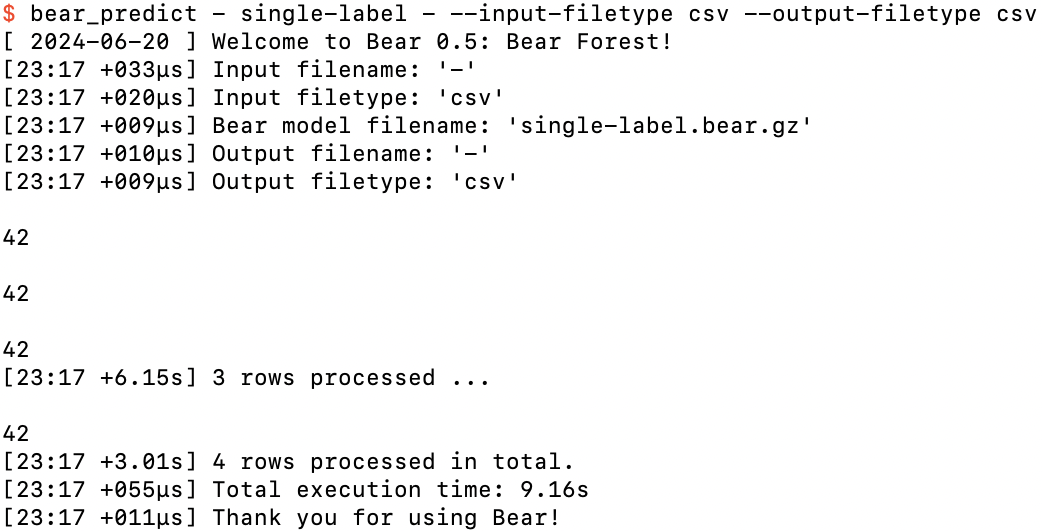
We can now run memory_bear on this dataset successfully:
Running memory_bear on single-label.csv
All of these steps will become clearer as we work through these tutorials, but we see that Bear built an “empty model.” It then “refreshed” and “finalized” the model, and then saved the “final Bear model” to single-label.bear.gz. If we take a look at the decompressed bytes in that file,
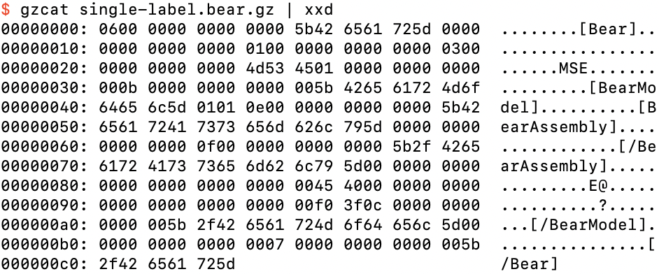
The bytes in single-label.bear.gz
we can see that it consists of binary data within plain text tags; this is the general way that Bear saves objects. It runs it through gzip to compress these 198 bytes down to 91.
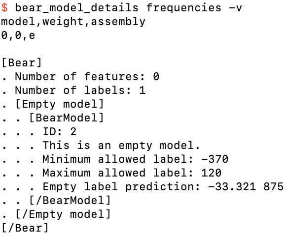
We can get an overview of what is in this model file using the supplied program bear_model_details:
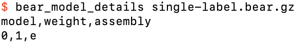
Getting an overview of single-label.bear.gz
That’s not too enlightening in this case! We can get a bit more detail using the --verbose option:
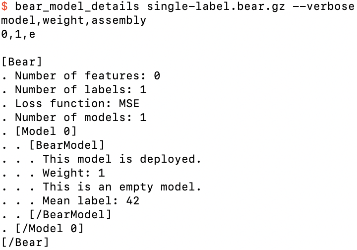
Getting some more detail of single-label.bear.gz
We can see the same [Bear] and [/Bear] labels that we saw in the binary file, but now the binary data between them is described in plain English. This printout of details actually uses the “debug print” functionality that is implemented throughout my codebase. Note that the tab indentations for nested content are also marked with dots, which makes it easier to parse these printouts for objects that are more complex.
Apart from the things that we specified to Bear, we see that there is just a single “empty” model, which is the model that Bear creates to model a label without using any features at all. This makes sense, because there were no features! This model is “deployed,” which just means that it’s not still in training. Its “weight” is 1, which makes sense because it is the only model! This empty model simply records that the mean label value in the training data was 42; that is all that empty models do.
We can now understand the non-verbose output a little better. There is only one row of data, for model 0 (the only model), with a weight of 1. The “assembly” “e” is simply shorthand for the empty model.
We can stream feature data through this model and get it to make predictions using the supplied program bear_predict. Its command-line options are similar to those of memory_bear:
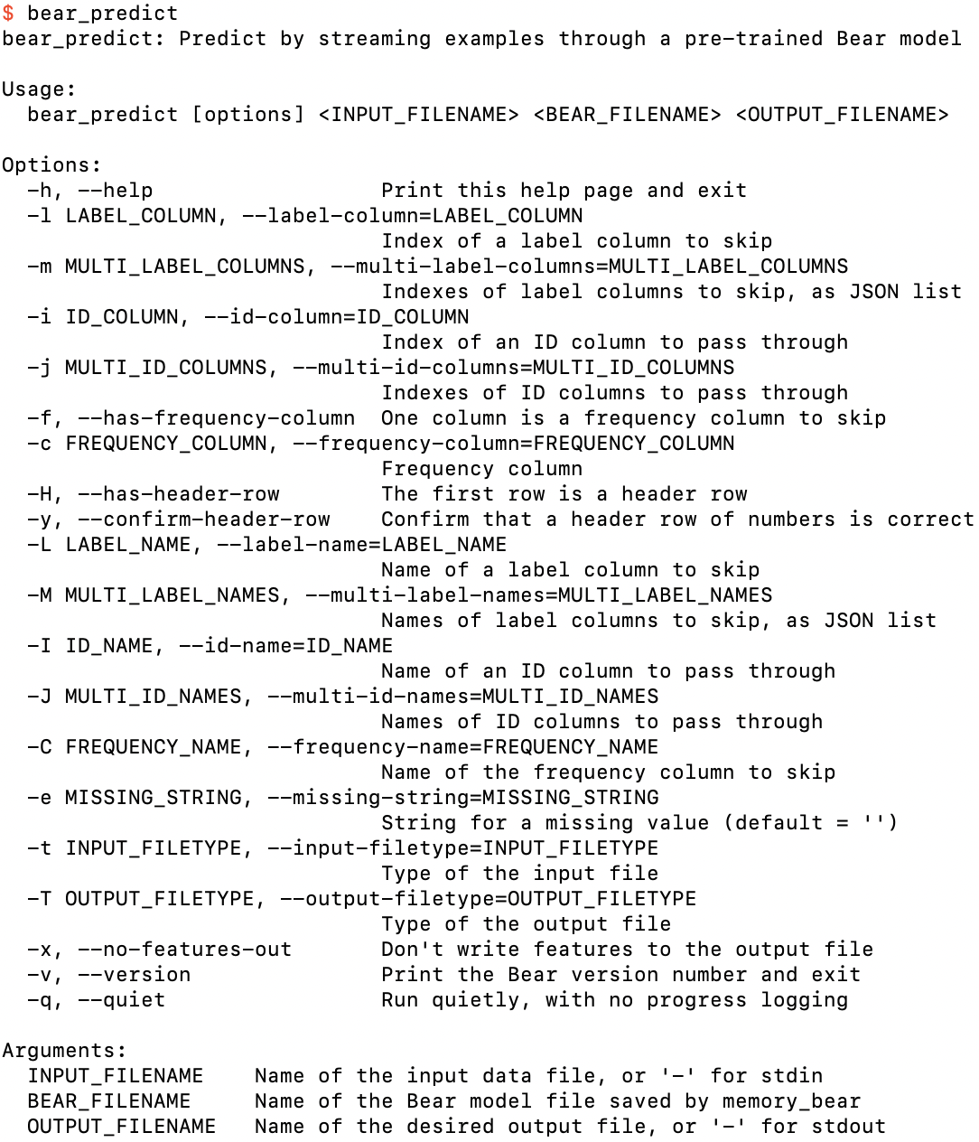
The help screen for bear_predict
As the argument specifications at the bottom of this help screen show, we can run it in “interactive” mode by specifying stdin and stdout for the input and output files (with the standard Unix convention of “-” for each), although we now need to specify the filetypes for each because there are no filenames that Bear could use to auto-detect what we want:
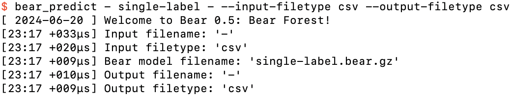
Running bear_predict on single-label.bear.gz in interactive mode
At this point, the program is waiting for us to specify feature values for an example. In this case there are no features, so if we hit the return key, it spits out its prediction:
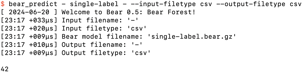
After hitting the return key
We can do this as many times as we want:
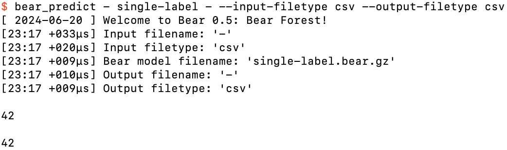
After hitting the return key again
If we’ve taken more than five seconds to do this, we'll even be given a “progress update” on the number of rows processed so far:
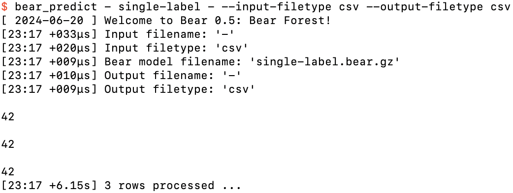
After hitting the return key a third time, more than five seconds after starting
After doing this a fourth time, the fun has probably worn off, and we can finish our input by pressing control-D and return:
Finishing our fun with control-D
Let’s make things slightly more interesting by having more than one example in our dataset. For example, 10-labels.csv:
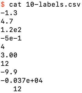
The data file 10-labels.csv containing 10 label-only examples
If we run memory_bear on this dataset, now using short option names,
$ memory_bear 10-labels.csv 1m -l 0 -s 10-labels
and look at the details of the model created, 10-labels.bear.gz,
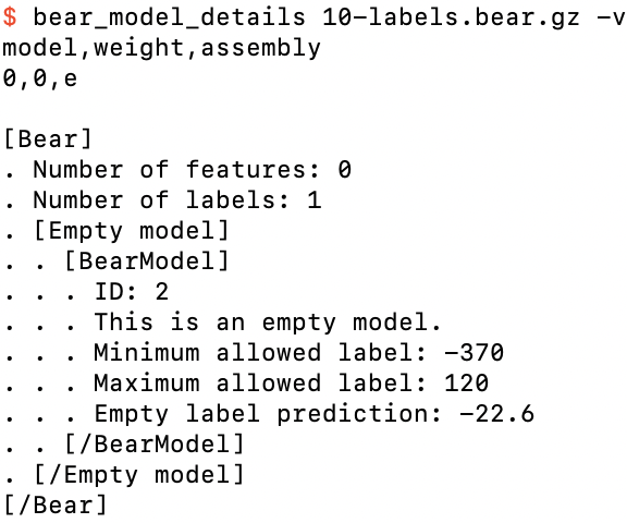
Details of 10-labels.bear.gz
we can see that the empty model now records that the mean label is −22.6.
As before, we can run bear_predict in interactive mode to stream example feature data (again, here we have no features) through the model:
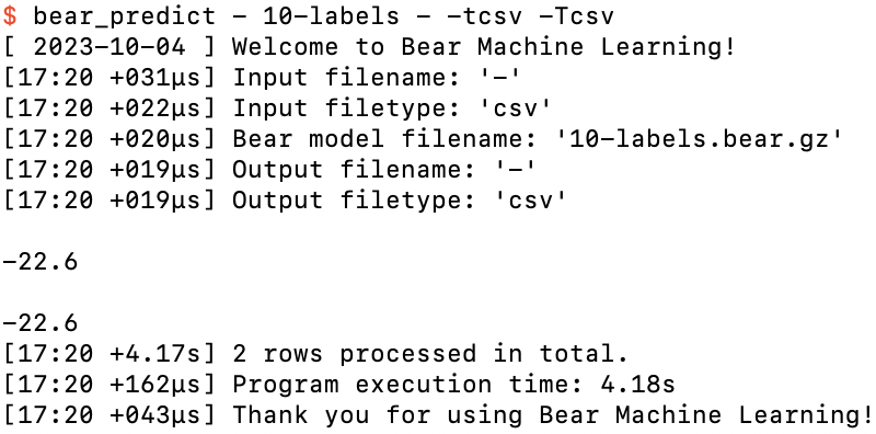
Running bear_predict on 10-labels.bear.gz
where this time our fun was expended after two hits of the return key, after which I hit control-D and return to end the input datastream.
Note that Bear’s prediction was the mean label value. The mean minimizes the MSE loss function, which is the default loss function for memory_bear.
What if we changed the loss function to something else—say, MAE:
$ memory_bear 10-labels.csv 1m -l0 -nMAE -s10-labels-mae
and run bear_predict on it:
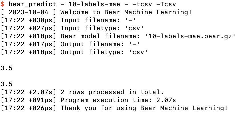
Running bear_predict on 10-labels-mae.bear.gz
The prediction is now totally different: 3.5. This is because the MAE loss is minimized when the prediction is the median label value, rather than the mean (or, technically, any arbitrary value in the closed interval between the two median values if there is an even number of data points). If you work it through, the median values for 10-labels.bear.gz are 3 and 4, and Bear has followed the normal practice of breaking the arbitrariness by taking the mean of these median values.
However, if we now look at the details of the model created, 10-labels-mae.bear.gz,
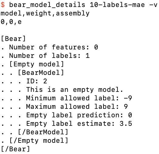
Details of 10-labels-mae.bear.gz
we see that things look wrong: the “mean label” is now listed as 0, rather than −22.6 (or 3.5, for that matter). What’s going on here?
The answer is that to support the MAE loss function, Bear performs a trick by transforming the label values under the hood into a quantity linearly related to their cumulative frequencies, which is what you need to use to compute the median. The way that I have defined that quantity automatically assigns the median a value of zero. Since the BearModel class is actually given these quantities rather than the original label values, it dutifully reports that their mean is zero (as it must be, by the way that this quantity is defined). At the end of the process Bear transforms these quantities back to actual label values, as we saw above when it gave a prediction of 3.5.
Ultimately, you don’t really need to worry about how Bear “makes the sausage” for loss functions other than MSE unless you are inspecting the details of the model file. In this case the “debug print” doesn’t actually give you all the data required to interpret the loss function’s transformation of the label values.
Let’s now add frequencies (counts of the number of examples having the given label value), to create frequencies.csv:
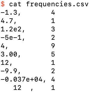
Adding a frequency column
This just means that we have 4 examples with a label value of −1.3, one example with 4.7, and so on. This is completely equivalent to having a data file with four rows with label value −1.3, etc.
We can specify that our input file has a frequency column by using the --has-frequency-column and --frequency-column options (here in their short forms -f and -c):
$ memory_bear frequencies.csv 1m -l0 -f -c1 -sfrequencies
which Bear parses and includes in its feedback to us:
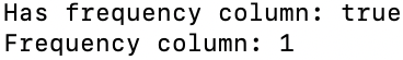
Bear’s feedback of our frequency column specifications
We now see that the model, frequencies.bear.gz, is similar to the previous one,
Details of frequencies.bear.gz
except that the prediction is now −33.321875. This is just the weighted mean of the input label values, where each weight is just the relative frequency; e.g., for the first label value of −1.3 it is 4 / 32, since the total frequency is 32; and so on.
Note that my codebase automatically includes separators (here, a space in the decimal value) in its logging, but these are never added in output files. We can confirm this by running bear_predict on the model:
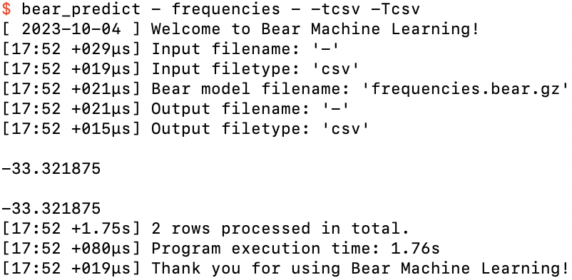
Running bear_predict on frequencies.bear.gz
Again, if we switch to the MAE loss function,
$ memory_bear frequencies.csv 1m -l0 -fc1 -nMAE -sfrequencies-mae
and check its predictions,
$ bear_predict - frequencies-mae - -tcsv -Tcsv
then we see that its prediction is now 3, which is just the (frequency-weighted) median of the values in frequencies.csv.
OK, enough with datasets with just labels and no features. Let’s add a feature!
The file bivariate-2.csv is a simple bivariate dataset (one feature and one label) with just two nondegenerate examples (i.e., the feature values aren’t equal and the label values aren’t equal):
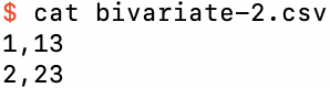
A simple bivariate dataset with two nondegenerate examples
This might seem to be a rather trivial dataset, but I’m going to spend some time on it, because it is illustrates the general process and philosophy of Bear Forest without being too complicated to visually parse.
Let us take the first column (column 0, with values 1 and 2) to be the feature, and the second column (column 1, with values 13 and 23) to be the label. Let us also give Bear 20 seconds for building new models:
$ memory_bear bivariate-2.csv 20s -l1 -sbivariate-2
You should see something like this:
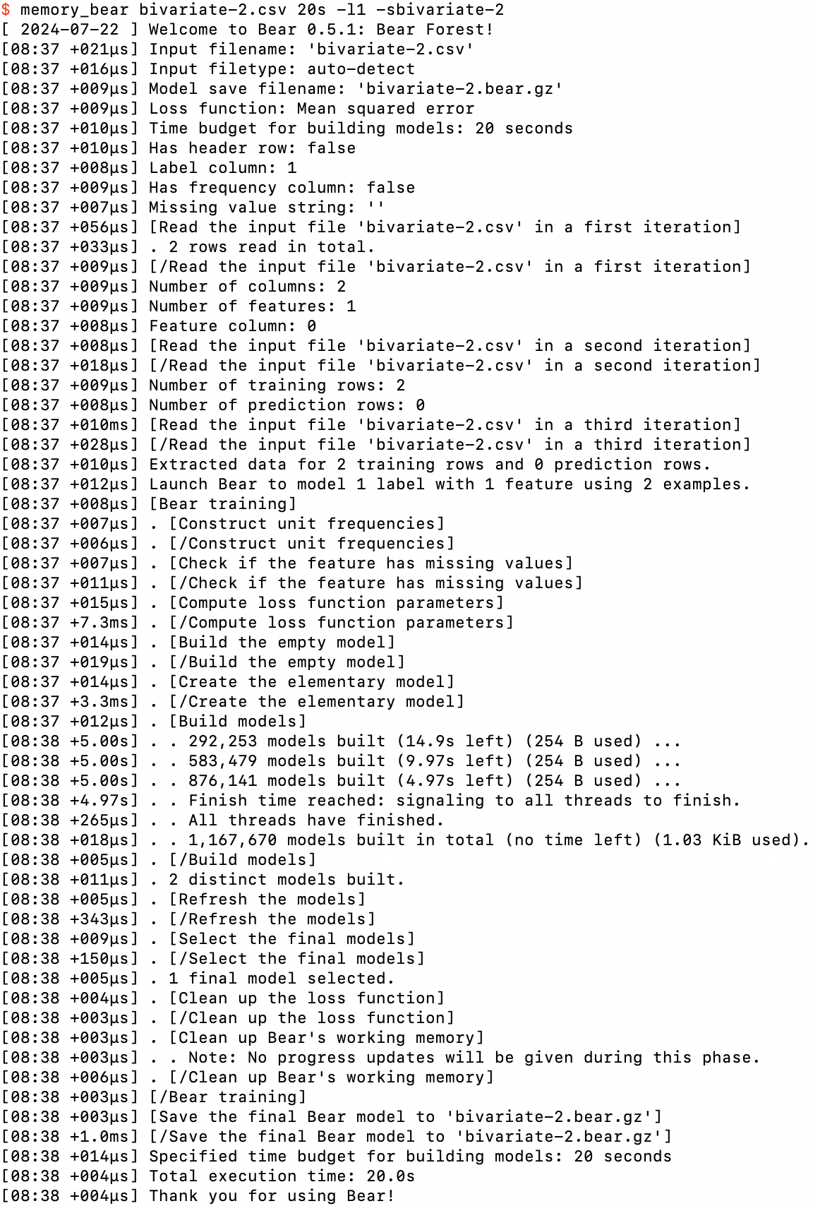
Running memory_bear on bivariate-2.csv
We can see two new phases here.
Firstly, after building the empty model, Bear creates the “elementary” model. An elementary model uses just a single feature to model the residuals of the empty model. Here we only have one feature, so there is only one elementary model. If we had more than one feature, Bear would create the elementary model for each of them in this phase.
Bear tracks the structure of each model—which features are being used to model the residuals of its parent model, and which features that model uses, and so on—by its “assembly.” We saw above that the assembly for an empty model is denoted e. The assembly for our elementary model is denoted e|0, which says that feature 0 (the first feature) is being used to model the residuals of the empty model. (If we had a second feature, its elementary model would be denoted e|1.) This modeling of the residuals of the empty model is called the first “part” of the assembly.
In general, Bear uses one or more features to jointly model the residuals of the parent of the given model. For example, the assembly e|0-1|5|0-5-17 represents Bear modeling the residuals of the empty model with features 0 and 1, and then modeling the residuals of that with feature 5, and then modeling the residuals of that with features 0, 5, and 17. This assembly has three parts: the first part has features 0 and 1, the second part has feature 5, and the third part has features 0, 5, and 17. Each part represents a model that models the residuals of its parent model.
This construction of more complex models happens in Bear’s “build models” phase. Each worker thread randomly chooses to either build a new model or “update” an existing model, which I will describe shortly. If it decides to build a new model, it constructs the assembly for the model it wishes to build by taking as a base one of the models it has already built, and then chooses a random part of the assembly of one of the other models it has already build as an “attachment” part. It then either “melts in” the attachment part by unioning the set of features of the attachment part into the last part of the assembly of the base, or else it “glues on” the attachment part to the end of the assembly of the base, as a new part modeling the residuals of the base. The base and attachment models are chosen at random from the models already constructed, but weighted towards those that have proven to be more useful than others in reducing the sum of squared residuals. Bear has a rule that no part can be repeated in an assembly, so if that happens to be the case for the assembly it has just constructed, it throws it out and tries again. Otherwise, it checks if it has already built the model corresponding to the assembly. If so, it “updates” it; otherwise, it builds it.
That’s the general situation. For our dataset bivariate-2.csv there is only one feature. Bear’s “no repeated part” rule means that if you only have one feature, there is only one possible assembly—and hence model—that it can build: the elementary assembly, e|0. Add that to the empty model and we have just two possible distinct models, which is exactly what Bear told us above that it found.
This means that all that Bear could do in the “build models” phase above was “update” the elementary model. In general, Bear updates a model by creating a new model that models the residuals of the parent model. But why should it need to create a new model if it has already created one?
The core modeling algorithm of Bear is somewhat complicated, and I probably will need to give a whole lecture on it one day, but in brief: it creates a “copula density hypercube” (a nonparametric representation of joint probability density) between all of the feature fields in the last part of the model’s assembly and the field of residuals of the parent model, and then merges adjacent “bins” along each field direction if it determines that the density hyperplanes orthogonal to each such bin are not statistically significantly different. Bear’s modeling process is therefore “frequentist,” in that it uses a statistical significance test in this decision, but it is also “Monte Carlo” in that it uses the probability of statistical significance to “roll the dice” to decide whether to merge or not. (It is also “Monte Carlo” due to randomly breaking any tie-breakers that it encounters in any part of the process.) Thus, similar to random forests, Bear will in general obtain a different specific model each time that it models a given set of parent residuals with a given set of features.
For my run above on my old M1 laptop, Bear built just over a million e|0 models in 20 seconds. Note that Bear tries to give you a “progress update” every five seconds or so, to assure you that it’s still working and hasn’t frozen up due to some bug. On each progress update it tells you how much time is left for building new models. It also tells you how much “swappable memory” has been used for the models; once this gets to a threshold amount (by default three-quarters of total system memory) it automatically swaps models out to storage; the progress updates will also tell you this, if and when it gets to that point. (This does not represent the totality of memory used by Bear, which in general is more difficult for Bear itself to determine, but it should represent the bulk of it.)
So let’s take a look at what Bear actually predicts using the overall model bivariate-2.bear.gz that it created from these million-odd models that it built:
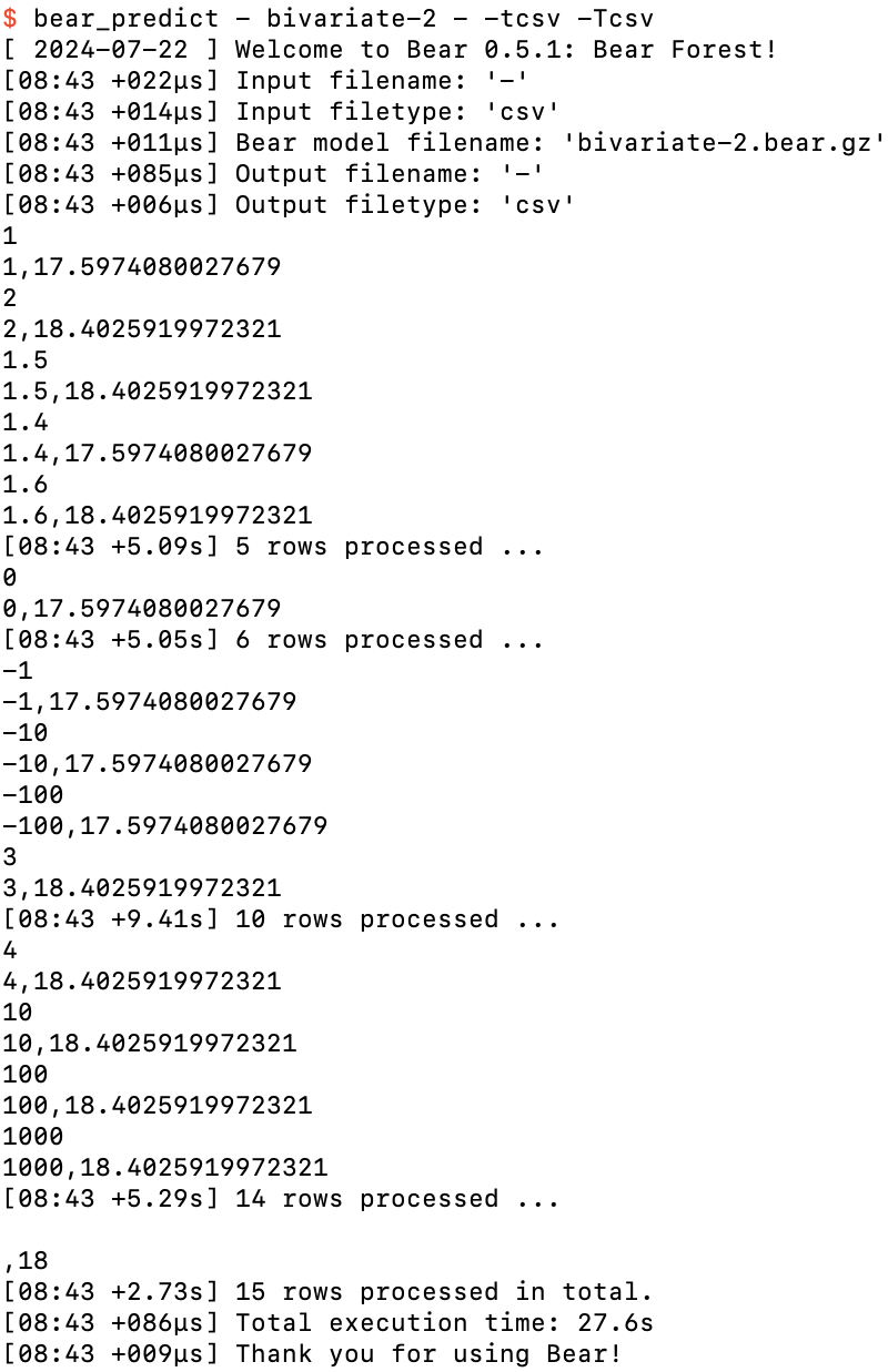
Ad hoc predictions from bivariate-2.bear.gz
Since there was one feature in the dataset we supplied to Bear, I needed to specify the value of that feature each time before pressing return. I started with the two feature values 1 and 2 that appeared in the training data. Bear’s predictions of 17.5974080027679 and 18.4025919972321 respectively were not identical to the label values in the training data (13 and 23), but they weren’t equal to each other either. It seems that Bear has “accepted a little bit” of the dependence of the label on the feature shown in the training data, but not all of it. I’ll return to this shortly.
After that I tried feature values between 1 and 2. Bear’s predictions were always one of the two values we saw above, jumping up somewhere around a feature value of 1.5. So then I tried feature values outside this domain: feature values less than 1 always gave the lower prediction, and feature values greater than 2 always gave the higher prediction. This is a general property of Bear’s models: they are piecewise constant. (I’ll also return to the question of exactly where it jumps up from the lower prediction to the higher prediction shortly.)
Finally, I hit return without specifying a feature value at all. Bear handles missing values such as this without a problem. You can see that its prediction in that case was just 18, which is the mean label value. This is the base prediction that it got from the empty model; without a feature value specified, the elementary model was not able to provide any prediction of the residual from the empty model, and so its overall prediction remained just 18. (Bear can also handle and model missing feature values in the training data, which we will see further below.)
So let’s now take a look at the model that Bear built:
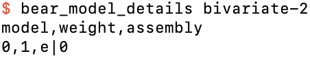
An overview of bivariate-2.bear.gz
We see the elementary model. But we saw that Bear actually had two models to consider in its final “Select the final models” phase: the elementary model and the empty model. It decided to not include the empty model at all. Its algorithm for selecting models is as follows. First, it always selects the model that minimized the loss function in training: that was the elementary model, which had a lower sum of squared residuals (SSR) than the empty model. It then figures out if adding in the next-best model—here, the only other model, the empty model—with a positive weight would reduce the overall SSR. (For example, if the residuals of two models are uncorrelated, then a suitable weighted sum of those two models will yield a lower SSR than either model taken alone.) In this case the empty model did not provide any improvement in SSR, no matter what weight it was added in with, and so it was not selected. (Of course, it is still the parent model of the elementary model, but it was not itself selected as one of the final models.)
Let us now take a look at the “verbose” details of the model:
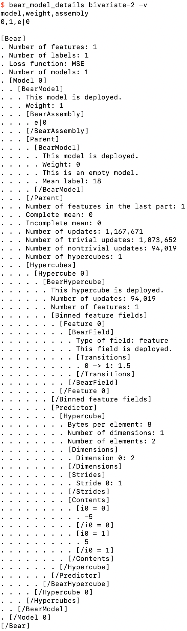
Details of bivariate-2.bear.gz
This is the last model that I will show in full detail like this; but, as promised, it is simple enough that I can now walk you through all of the parts of it, so that you can gain some understanding of how Bear’s modeling process works.
The top of the printout looks the same as what we had above. But now the single model has an assembly of e|0 rather than e. After its assembly we see a complete embedded printout of the details of its parent model, the empty model. The mean label is 18, as we noted above. We then see the details of the elementary model itself. It has one feature in its last part. The “complete mean” and “incomplete mean” will be of interest to us later; suffice it to say that they are both zero here.
We then see that this model contains 1,167,671 updates, corresponding to the 1,167,671 models that it built in training, with 1,073,652 of the updates being “trivial” and the remaining 94,019 of them being “nontrivial.” A “trivial” update is one for which Bear’s algorithm has reduced the copula density hypercube (here a 2×2 square) down to one single big hypercell covering the whole hypercube (here the whole square); in other words, all possible merges of adjacent bins were ultimately done. This is what happened here nearly 92% of the time: the 2×2 square was reduced down to a single square; the two feature value bins were merged, as were the two label value bins. But because Bear’s algorithm is Monte Carlo frequentist, the other 8% of the time it did not merge these bins.
For those 8% of updates, Bear constructed a BearHypercube object. We can see that it tracks the fact that it had 94,019 updates; in other words, each of those 94,019 updates created exactly the same hypercube structure. (With a 2×2 square, that’s the only nontrivial possibility; in general there will be many possible structures for the reduced hypercube.) It then tells us that it has one feature field, and shows us details of the BearField object for that feature field, which tracks information for the binning of each field. Here, in its final “deployed” form, it tells us that the transition from bin 0 to bin 1 happens at a feature value of 1.5, which agrees with we what we saw above when we played with bear_predict. It then gives us details of its “predictor,” which is just a hypercube of all the combinations of feature bins, each hypercell of which contains the prediction of the parent model’s residuals for that feature hyperbin. Here we see that if the feature is less than 1.5, it predicts −5; if the feature is greater than or equal to 1.5, it predicts +5.
So if we took that hypercube alone we would see that it “predicts” the input examples perfectly: adding −5 or +5 to the empty model’s mean label value of 18 gives us back the label values 13 and 23 of the input dataset. But Bear does not use just this hypercube when making predictions from this model: it also takes into account the fact that that hypercube was only estimated to be statistically significant just over 8% of the time. The other nearly 92% of the time the hypercube was found to be trivial, and the model just falls back to the empty model prediction of 18. Bear weights each update equally, so the amount added to the empty model’s mean label of 18 is just 94,019 / 1,167,671 (or 8.0518399446419%) of ±5, which is ±0.402591997232097, which is just what we saw above.
So you might ask: why does Bear decide the hypercube is trivial around 8.05% of the time, and what exactly is the precise value of that percentage?
I will answer both of these questions in the advanced tutorial. But to at least get a better empirical handle on the second question, I ran Bear on my laptop for three hours, and got this from bivariate-2-3h.bear.gz
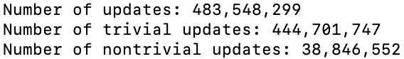
The number of updates found for bivariate-2 from a 3-hour run on my laptop
That tells us that the true percentage of nontrivial updates should be (8.0336 ± 0.0024)% with 95% confidence, if we use the Normal approximation to the Binomial distribution.
We saw above that the prediction jumps up from its low value to its high value at a feature value of 1.5, which makes sense as the mid-point between the two feature values of the two training examples; and Bear’s model file confirms that that is where it makes the transition. But if you play around with bear_predict with either bivariate-2 model and bisect to figure out where it actually jumps, you might be surprised to find that it doesn’t happen at a feature value of 1.5, but rather at around 1.498046875. What’s going on here?
The answer is that Bear internally uses a custom 16-bit floating point representation, that I dubbed “paw,” in the core engine that does the statistical modeling. The paw format is very similar to Google Brain’s bfloat16 format, except that paw has 7 bits of exponent and 8 bits of mantissa, whereas bfloat16 has 8 bits of exponent and 7 bits of mantissa. Google chose one less bit of precision that I did for Bear because they had competing design goals due to a legacy codebase that made it advantageous for bfloat16 to have the same dynamic range as the standard 32-bit float. I had no such constraints, and could let paw have one extra bit of precision, since the dynamic range of paw of around 10±19 is more than sufficient for all practical purposes, compared to around 10±38 for bfloat16.
The result is that feature values greater than 1.5 − 1 / 512 round up to 1.5 in this core modeling.
But the fact that the paw floating-point type is only “half-precision” raises a potentially troubling question: what if our two feature values were “shifted right” by, say, a million? For example, bivariate-2-shifted.csv:
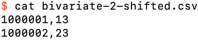
The dataset bivariate-2.csv shifted right by 1,000,000
You might guess that the two feature values would now be quantized to the same paw value, and so would always be “binned” by Bear into the same bin. But if you run Bear on this dataset, you find that it still finds the same model as above. How did it manage this?
The answer is that Bear first analyzes the distribution of values for each feature field, and if the domain is further away from zero than the “width” of the domain (its support), it automatically “offsets” that feature by the midpoint of the domain, so that all feature values sent to each Bear hypercube (which is the thing that converts them to paw values) are relative to this midpoint. (Residuals are “automatically offset,” because the empty model removes their mean.) In this particular case, the transition now occurs at exactly 1,000,001.5, because this is the midpoint offset value, and the paw format is still floating point, i.e., retains dynamic range around zero. (With more than two feature values the transitions would again be more obviously quantized; this is a special case.) If you look at the details of the model file bivariate-2-shifted.bear.gz, you will see that the BearField contains the details of this offset:
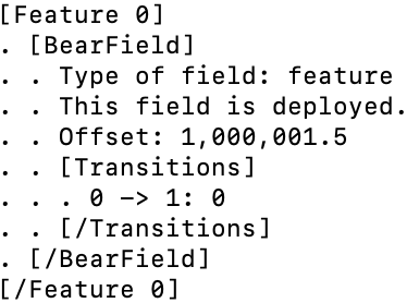
Details of a BearField with an offset
where now the transition between bins occurs at an offset feature value of 0, i.e., at an actual feature value of 1,000,001.5.
We might seem to be progressing rather slowly towards real-life datasets, but bear with my baby steps a little longer. Let us add a third datapoint to our bivariate dataset, collinear with the first two (with no noise), in collinear-3.csv:
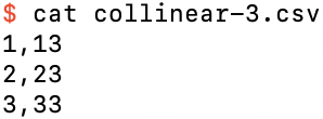
Three bivariate examples in a noiseless straight line
If you run Bear on this dataset, creating collinear-3.bear.gz, you might be disappointed to find that it finds even fewer nontrivial updates than the above case: about 0.9% of updates. But this is not a bad thing: there is really very little statistical significance in just three datapoints. Bear now finds three different nontrivial hypercubes: one with a single transition between feature values 1 and 2 (about 49% of nontrivial updates), another with a single transition between 2 and 3 (another 49%), and one with two transitions, between all three feature values (the other 2%). Overall, the difference in its label prediction as the feature value is increased from 1 to 2 or from 2 to 3 is about 0.07.
One way to add more statistical significance to this dataset is to specify that each example has a frequency greater than one. For example, we can specify that each has a frequency of 2, in collinear-3-f-2.csv:
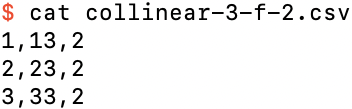
Adding more frequency to each row of collinear-3.csv
The resulting model file collinear-3-f-2.bear.gz now has around 25% of updates being nontrivial. Of course, we have done this by doubling the total frequency (really, the total number of examples) in the dataset, from 3 to 6, but at least it is getting there. Now the difference in its label prediction as the feature value is increased from 1 to 2 or from 2 to 3 is about 2. That’s still a factor of 5 less than the variation shown in the input data (which has a gradient of 10, not 2), but, again, we only have a total frequency of 6 here.
We can jump to an even greater amount of significance by bumping up the frequency of each example to, say, 10, as in collinear-3-f-10.csv. We now see that Bear obtains an almost perfect model for this dataset. Of course, the training data here is completely noiseless, with the label being a function of the feature, with enough frequency for each data point that Bear is able to almost perfectly match that noiseless data.
In the above I used bear_predict in interactive mode, entering each “test” or “prediction” example of features (in the above cases, either no features at all, or just one feature) on the keyboard and hitting return each time. You can of course also stream a file of test rows through your model to obtain its prediction for each test row.
For example, consider collinear-3-f-10-test.csv:
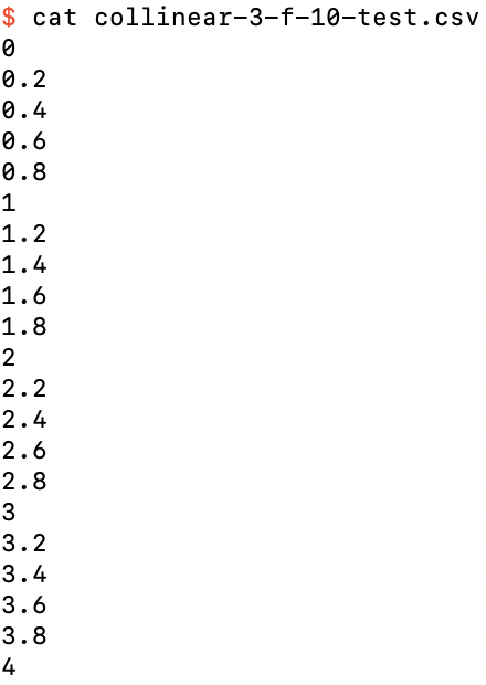
The file collinear-3-f-10-test.csv of test rows
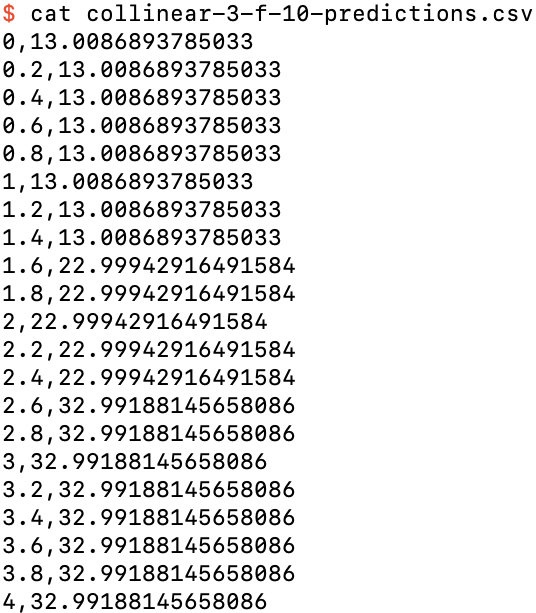
We can stream this file through our model, collecting the predictions in the output file collinear-3-f-10-predictions.csv:
$ bear_predict collinear-3-f-10-test.csv collinear-3-f-10 collinear-3-f-10-predictions.csv
The results are just as we expect: a piecewise constant model, which in this case models the three training examples almost perfectly:
The file collinear-3-f-10-test.csv of test rows
You can also graph this dataset using any program you like. Here I’ve just used Excel, for simplicity:
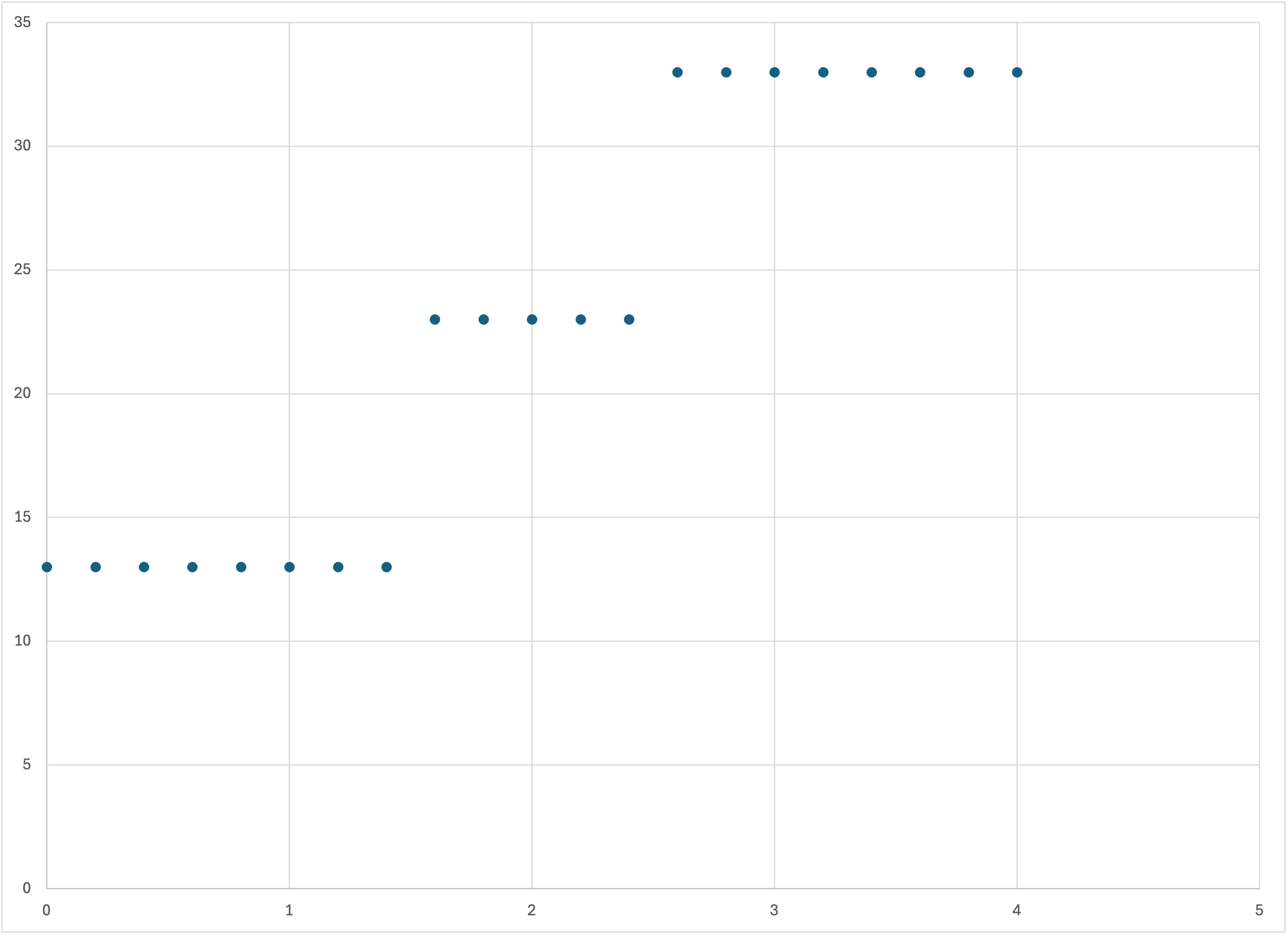
Plot of the predictions collinear-3-f-10-predictions.csv using Excel
As a convenience, memory_bear lets you include prediction rows (test rows) in the same input file as your training data, and it will make predictions for those rows after it finishes creating its model. All you need to do is include those rows in your input file with an empty label field. For example,
$ cat collinear-3-f-10.csv collinear-3-f-10-test.csv > collinear-3-f-10-combined.csv
simply appends the test rows to the training rows. The label values in column 1 are implicitly missing for the test rows (since there is no column 1), which marks them as prediction rows. Frequencies are never needed for prediction rows, so it doesn’t matter that column 2 is also missing for these rows.
We now have to specify an output filename for the predictions to be written out to. (In this mode, it is optional whether you want to save the Bear model to a file or not.) So the command
$ memory_bear collinear-3-f-10-combined.csv 20s -l1 -fc2
-ocollinear-3-f-10-out.csv
trains the model on the three training rows and then makes predictions for the 21 test rows, writing the results of those predictions out to collinear-3-f-10-out.csv. (The model is not saved; it is used for the predictions, and then discarded. If you want to save the model, specify the model filename as above.)
Bear also allows you to specify that one or more columns in your input data file should be simply passed through as plain text to the corresponding row of the output file, without playing any role in the actual modeling or predictions. This can be useful if one of your columns is a primary key, or if multiple columns together form a composite primary key, or even if some columns are simply comments or other descriptive text. For example, if we add an identifier column and a comment column to collinear-3-f-10.csv, and add a few prediction rows, to create ids.csv:
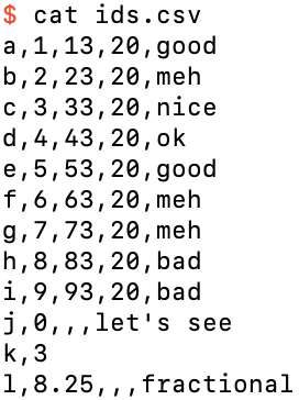
The data file ids.csv
and then specify to memory_bear that columns 0 and 4 are “ID” (passthrough) columns,
$ memory_bear ids.csv 1m --multi-id-columns='[0,4]' -l2 -fc3 -o ids-out.csv
then we can see that these two columns are ignored for training (they are considered to be neither features nor labels; they are just ignored), but they are passed through for the prediction rows to the output:
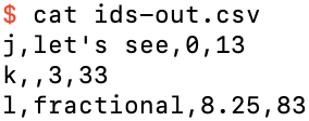
The output file ids-out.csv
If you specify one or more identifier columns in this way, you may not actually need or want to see the actual feature values for those rows. To suppress their output you can just specify --no-features-out:
$ memory_bear ids.csv 10s -j'[0,4]' -l2 -fc3 -o ids-out-nf.csv --no-features-out
Now in the output you just see your ID columns and the corresponding predicted label:
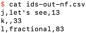
The output file ids-out-nf.csv
Although you can specify to memory_bear and bear_predict any arbitrary columns to be labels or identifiers, both programs write out predictions with all identifiers first, followed by all features (unless specified otherwise), followed by all labels, in each case in the order that the columns appeared in the input data. If you need an alternative permutation of the columns in the output file you should use another utility to achieve that result.
We’ve played enough with our noiseless collinear datasets, so let’s generate some data that at least has some noise added to it. You can do this yourself using whatever program you like, but I’ll use the supplied program simple_bear_tutorial_data so that you have the same data:
$ simple_bear_tutorial_data linear-50.csv -r19680707
which by default creates a file (here we have specified the filename linear-50.csv) with 50 training rows and 250 prediction rows in it. The final argument -r19680707 simply ensures that you seed the random number generator the same as I did, so that you get exactly the same data. If you graph the data you should see something like this:
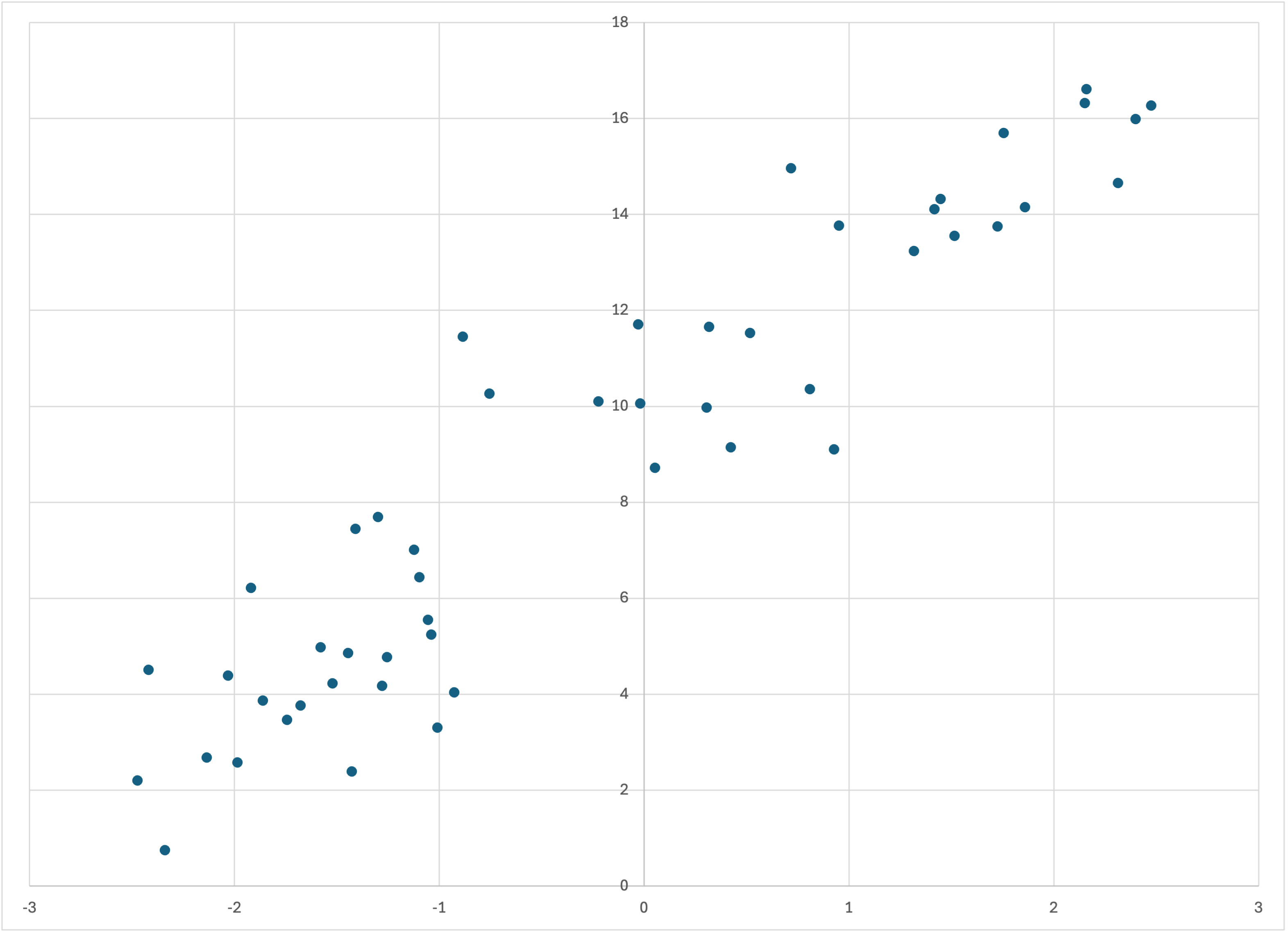
Scatterplot of linear-50.csv
Now run memory_bear on this data, giving it, say, 10 seconds for building new models:
$ memory_bear linear-5.csv 10s -l1 -o linear-50-predictions.csv
Graphing linear-50-predictions.csv (again, I will continue to use Excel for simplicity), you should see something like
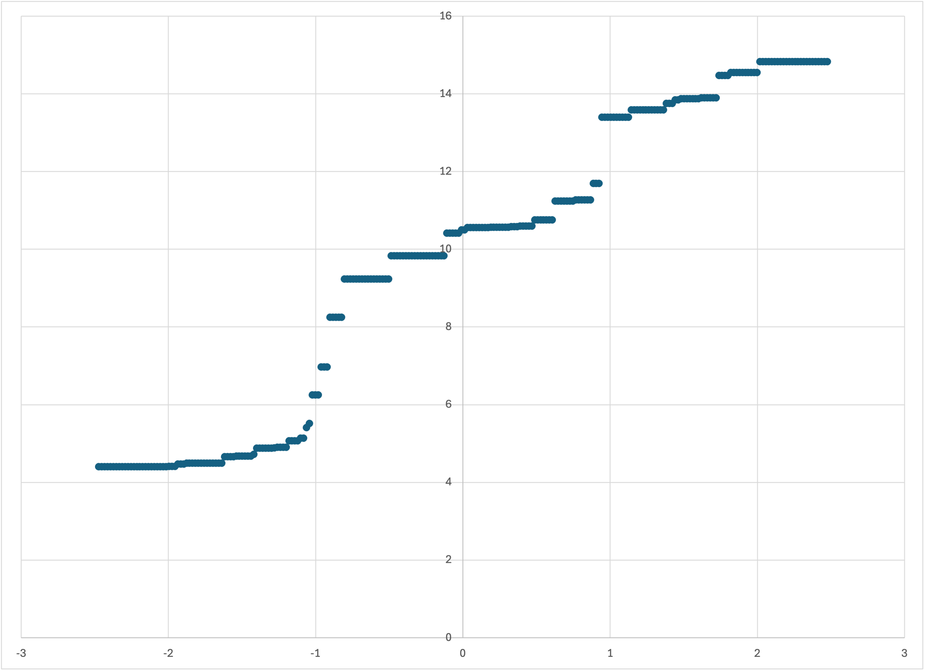
Scatterplot of linear-50-predictions.csv
This is our first nontrivial and nonpathological application of Bear, and arguably the results are, at first sight, somewhat intriguing.
Firstly, the model seems to have ignored the “noise” in the training data, but has just followed its “trend.” This is, of course, exactly what we want, but it’s somewhat startling to actually see Bear doing it. (I was surprised myself to see this result when first getting Bear Forest running in June 2024; I did not expect it.) Of course, the model is piecewise constant—as Bear’s models always are—but the “jumps” in it are arguably quite reasonable, given the relatively small amount of data (just 50 training examples) that this model is based on.
Secondly, the model is non-decreasing: you can confirm from the actual output file that the piecewise constant prediction pieces jump up as you go from left to right, never down. There is nothing in Bear that ensures this; indeed, we will soon see models in which it is not true. And, in fact, I haven’t even told you yet how the training data was created, so it’s not even clear that Bear’s model is even reasonable (maybe it should have been bouncing around like the training data?).
Thirdly, it seems like Bear’s model follows the trend of the training data fairly well everywhere except at the ends, where it looks like it “flattens out,” whereas the training data still seems to be trending with a positive gradient.
It would be nice to be able to see Bear’s predictions on the same axes as the input data. The memory_bear program lets you do that, by using the --debug flag:
$ memory_bear linear-50.csv 10s -l1 -d -o linear-50-debug.csv
Opening linear-50-debug.csv, you should see that the first 250 rows are just the same as linear-50-predictions.csv (but the precise prediction values will be slightly different because they come from two different runs of Bear). The next 50 rows are just the original training data, with the second column left blank but the third column containing the label value; the reason for this will be clear shortly. Following that are two extra columns, containing the prediction of the model for that training row, and the resulting residual.
Now, if we graph just the first three columns (i.e., the first is the ‘x’ value, and the second and third are two different data series for ‘y’ values), we get just what we wanted:
Scatterplot of the first three colummns of linear-50-debug.csv
We see more clearly that our observations were correct: Bear’s model does a good job of going “down the guts” of the data for most of it, but flattens out towards the ends and fails to keep following the trend of the data.
How can we understand this behavior—both the good and the bad?
I believe that they both come from the fact that each hypercube that Bear creates is piecewise constant, with each piece being, on average, statistically significant. Any single such hypercube may be a relatively “rough” approximation to the true trend of the data, in that it only has a relatively small number of pieces. Indeed, if we also save the model file,
$ memory_bear linear-50.csv 10s -l1 -d -o linear-50-debug.csv -slinear-50
and inspect the results,
$ bear_model_details linear-50 -v
(be patient: you will likely have thousands of hypercubes in the output!), you will see that each hypercube generally has between 2 and 6 pieces, with the most common being 3 or 4. I visualize these pieces as being like horizontal sticks, so that most of these individual hypercube models have just three or four of these sticks. Indeed, before Bear Forest, this is all that Bear could do. But by allowing a forest of hypercubes for each model, Bear averages out a large “bundle” of sticks around each feature value. This averaging is what allows the overall model to follow the trend of the underlying data, without bouncing around with its noise—since none of the sticks in the bundle do. (I am sure that there is a technical term for “a bundle of sticks,” but for some reason I don’t think that it would be advisable for me to use it in my technical description of Bear.)
This “bundle of sticks” visualization explains why Bear generally does a good job: at any feature value, it is averaging out the right ends of sticks that lie mainly to its left, the middles of sticks that are pretty well centered on it, and the left ends of sticks that lie mainly to its right. It is a little like a moving average, but also fundamentally different: at places where the training data jumps up drastically, most or all of the hypercubes will have a breakpoint, i.e., sticks to the left of that point will end there and sticks to the right will start there; there are no sticks that straddle that value. The result is that the overall average also jumps up at that point, as we see above at a feature value of just below 1.
This also explains why Bear ceases to follow the trend of the data as you get towards the ends of the domain of feature values. As you get to feature values toward the left edge, there are no sticks that lie mainly to the left, because there are no longer enough data points to the left to create such sticks in a statistically significant way. So the leftmost portion of Bear’s model largely consists of sticks that extend to the left edge, i.e., are the “first” stick for each hypercube, reading left to right. As we move to the right, we slowly start bringing in the “second sticks” for some hypercubes. And then eventually we reach the “steady state” mode where there is a variety of sticks to the left, across the middle, and to the right (except where the data jumps suddenly), where Bear’s average is able to track the data in a more “balanced” way.
Let’s now return to an important question: how did the simple_bear_tutorial_data program create this dataset in the first place?
Well, I gave some of that away by calling the dataset “linear-50.” The underlying analytical form of the data is a straight line, by default y = 3 x + 10, as you can find by running the program without any arguments. The x values are chosen randomly, uniformly between −2.5 and +2.5. To the corresponding y value is added normally distributed noise with standard deviation 1.5.
If you look back up at the original scatterplot above, this linear trend plus gaussian noise makes perfect sense. But Bear’s model was by no means a straight line, but rather a snaking sort of trend line with jumps in it. Does Bear’s model make sense?
I think it does. Bear was not in any way told that the underlying signal was a straight line. All that it had was the training data, and was asked to infer any trend that it could discern, in a nonparametric way. If you were given the training data above, and told that the true underlying functional form of the signal could be arbitrarily complicated, including step functions, then I think that your “best guess” of the underlying functional form would not be too far from Bear’s model, except at the ends.
In any case, this is what Bear does, for good or for bad.
We’ve seen that Bear has done a reasonable job of modeling noisy data with a linear dependence with 50 data points. But is that specific to the particular dataset that I created above? What if we change the random seed? For example,
$ simple_bear_tutorial_data linear-50a.csv -r19660924
which creates the dataset
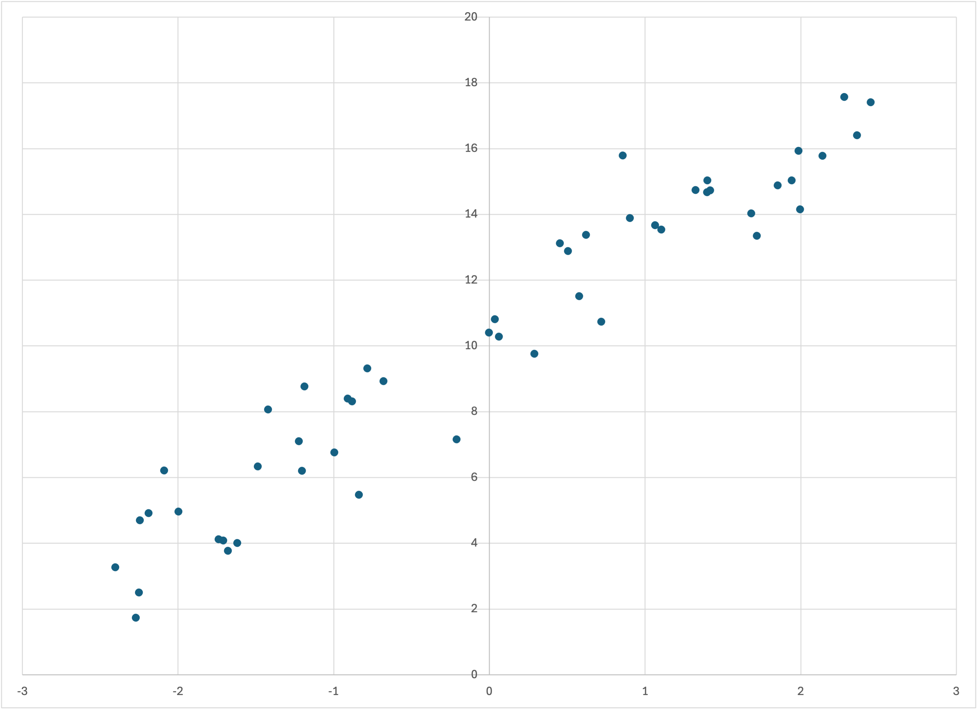
Scatterplot of linear-50a.csv
which actually looks a little “smoother” than linear-50.csv. (Of course, this is all just due to the random noise.) Running Bear on this dataset,
$ memory_bear linear-50a.csv 10s -dl1 -olinear-50a-predictions.csv
we see in linear-50a-predictions.csv that Bear’s model—like the training data—is a little bit more “linear” (again, except at the ends, where Bear conservatively does not “go out on a limb” for those last few data points):
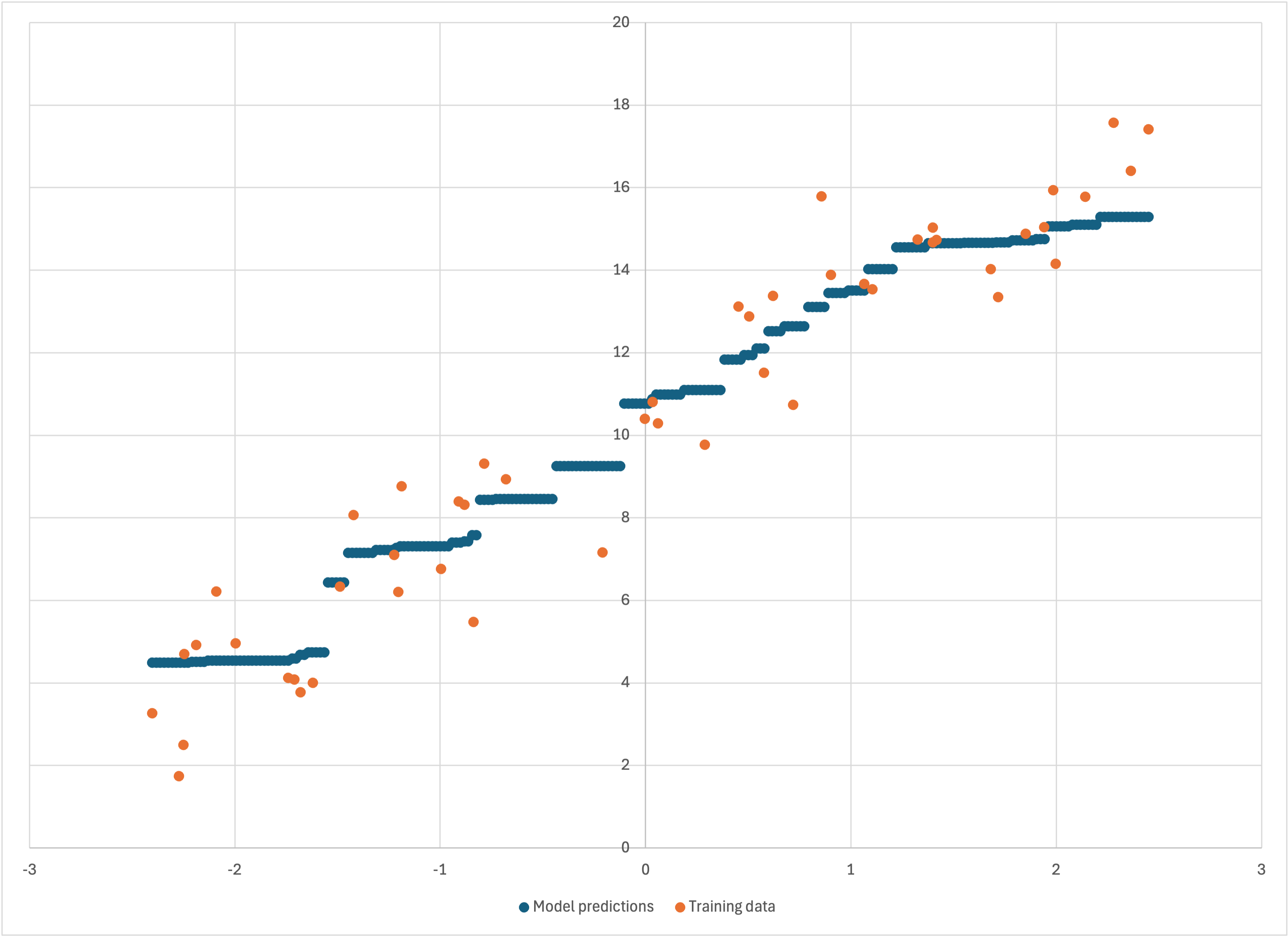
Scatterplot of linear-50a-predictions.csv
We can also look at what happens when we add more training data. Let’s return to the original random seed, and specify that we want 1000 rows of training data rather than the default 50:
$ simple_bear_tutorial_data linear-1k.csv -r19680707 -t1000
which creates
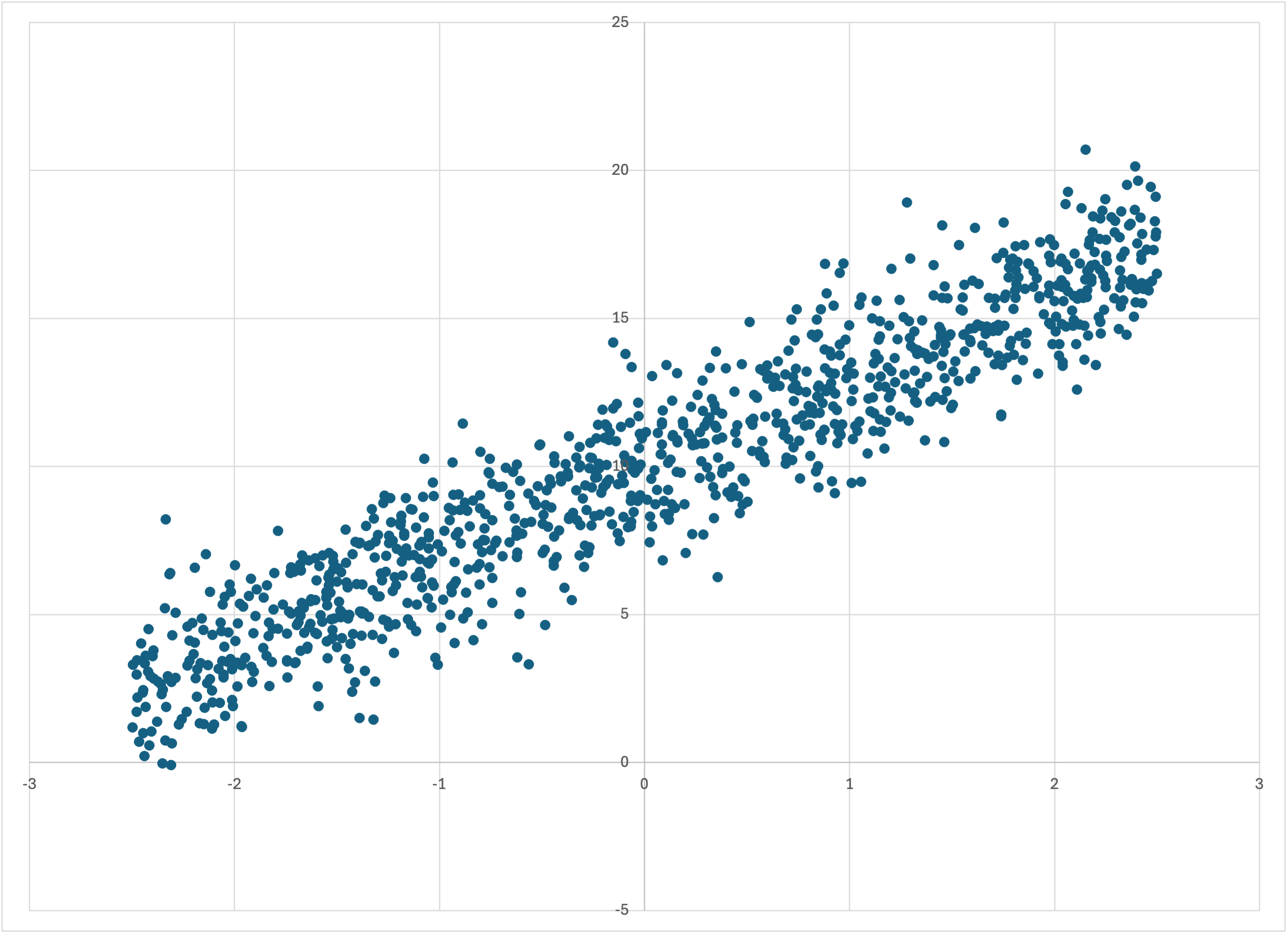
Scatterplot of linear-1k.csv
Running memory_bear,
$ memory_bear linear-1k.csv 1m -dl1 -olinear-1k-predictions.csv
now yields

Scatterplot of linear-1k-predictions.csv
where I have reduced the dot size so that the data can all be seen. Bear’s model is smoother, but it still seems to “staircase” along somewhat—even if that’s now a “worn staircase.” You might wonder: did Bear do this simply because we didn’t give it enough time to build enough models, or is this really what Bear’s best estimate of the underlying signal is? Bear built over 4,000 models in those 10 seconds, which seems like a lot—but we did have 1,000 data points, compared to only 50 previously.
To answer this question, I ran Bear again on this dataset, now with 5 minutes for training rather than 10 seconds, yielding nearly 100,000 models. The resulting linear-1k-predictions-5m.csv looks so identical to what is shown above that there is no point in me showing it to you separately.
So, for a given dataset, and a sufficient amount of time, Bear will converge on a single model that is its “asymptotic estimate”; i.e., what it would obtain if it had an infinite amount of time for modeling. That asymptotic model should not be “distracted” by the noise in the training data. It will produce what it believes is its best estimate of the underlying statistically significant signal. But that estimate will depend on the particular set of noisy data that it has been given. A different dataset from the same underlying signal but new random noise will lead to different “wiggles” in Bear’s model. Bear can only follow the data that it has been given, which as far as it is concerned may have come from any imaginable underlying signal.
It is also worth looking more quantitatively at whether Bear underfits or overfits the data it is given. It seems, visually, that its models are in the “Goldilocks” zone of being “just right,” but it is worth putting some quantitative numbers behind those observations. We know that the simple_bear_tutorial_data program added gaussian noise with a standard deviation of 1.5 to every label value. Working with the residual columns in linear-50-debug.csv and linear-1k-predictions.csv, we find that the standard deviation of the residuals is 1.61 for the former and 1.55 for the latter. These heartening calculations give us confidence that Bear is pretty well doing the best it can, with it doing a slightly better job the more data it has. (The edge effects noted above likely account for much of this variation: the standard deviation of the residuals for the middle 40 of the 50 data points for linear-50 is also 1.55.)
In the real world you will often be missing data for some features for some examples. Bear handles missing feature values.
To see how this works, let’s create a dataset like linear-50.csv, but with around half of the rows having a missing feature value. We can do this using the --missing-percentage option to simple_bear_tutorial_data:
$ simple_bear_tutorial_data missing-linear.csv -r19680707 -n50 -t100
where -n50 sets this “missing percentage” to 50%. I’ve also upped the total number of training rows to 100 so that about 50 of them will still have feature data. Indeed, if you inspect missing-linear.csv you will see that there are label values for the first 100 rows, but for 55 of them there is no feature value:
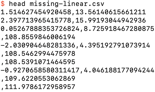
The first 10 rows of missing-linear.csv
Note that the label values for examples with missing features are clustered around 110. This is because the --missing-bias default is 100, which is an extra bias added to the label of all rows with a missing feature value, in addition to the default --bias of 10, so that the expectation value of the label for examples with a missing feature is 110. (The default --weight of 3 does not come into play, because there are no feature values to be correlated with for these examples.)
Usually, after the training examples we see the test (prediction) examples. But in this file we see a row with no values at all:
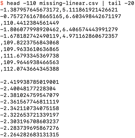
The 91st through 110th row of missing-linear.csv
This is actually a test row (since its label is missing), but for the case when the feature value is missing. After this row are the standard 250 test rows that the program has given us each time.
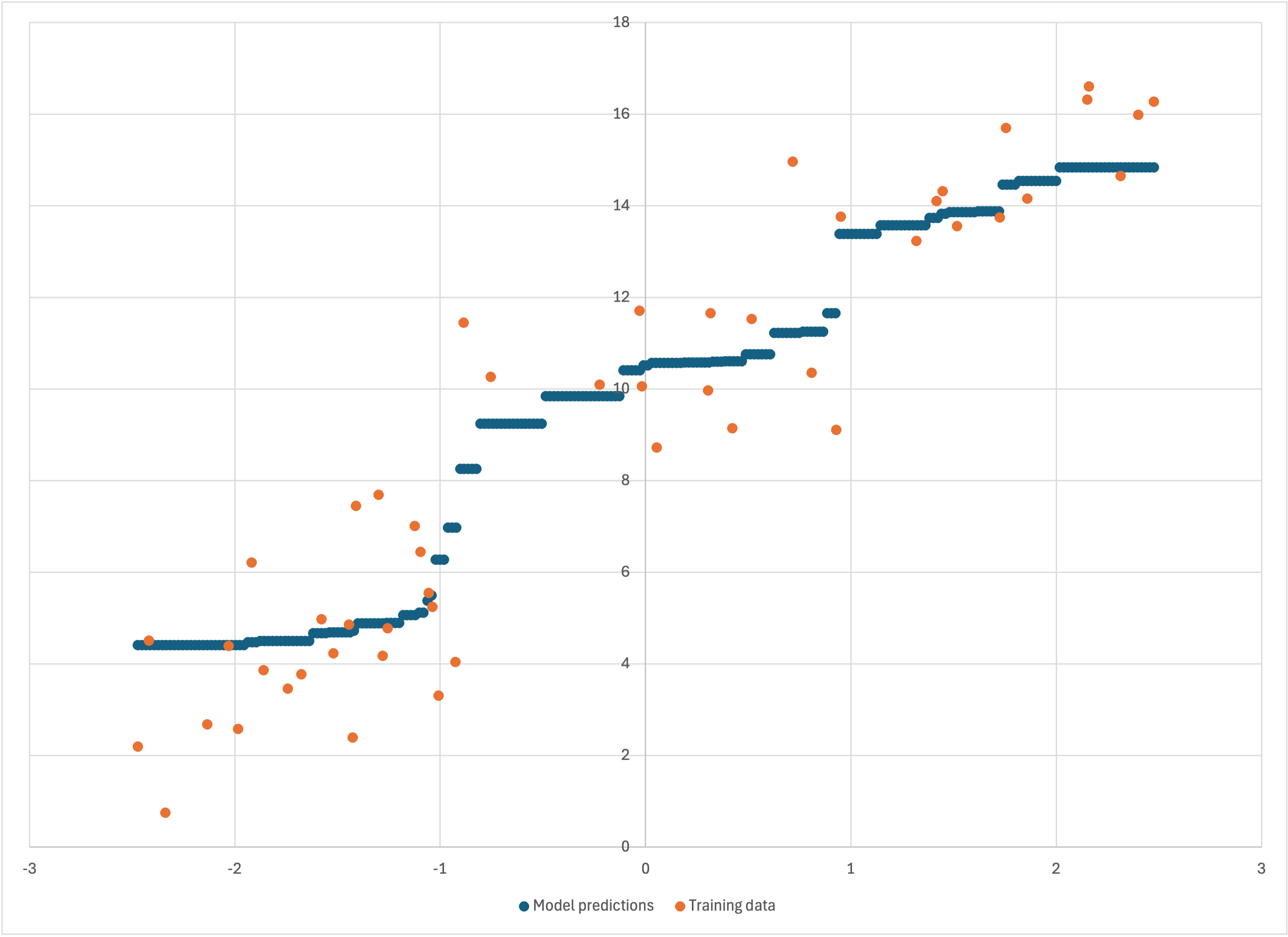
If you graph the 45 examples in missing-linear.csv that do not have a missing feature value, you will see that they follow the same general pattern as linear-50.csv and linear-50a.csv:
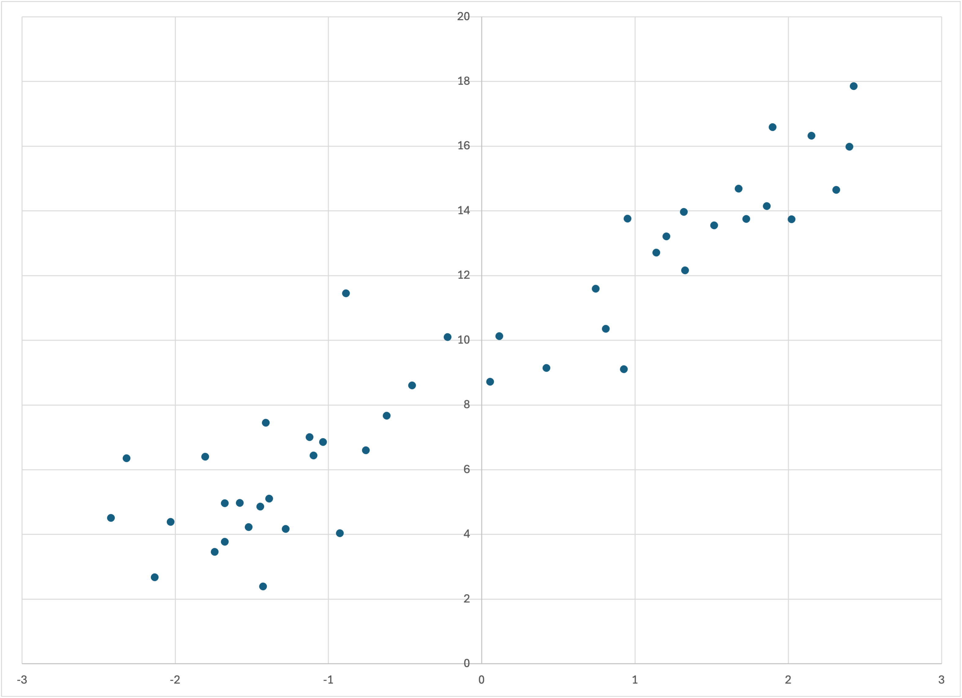
The 45 training examples in missing-linear.csv that do not have a missing feature value
Running memory_bear on this data,
$ memory_bear missing-linear.csv -dl1 10s -omissing-linear-predictions.csv
we see from missing-linear-predictions.csv,
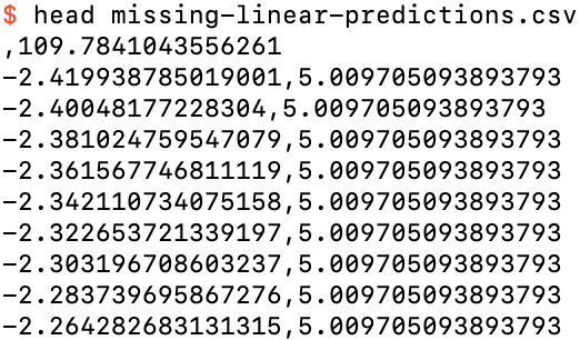
The first 10 rows of missing-linear-predictions.csv
that the prediction for a missing feature value is almost 110, and if we graph the predictions for the examples without missing feature values,
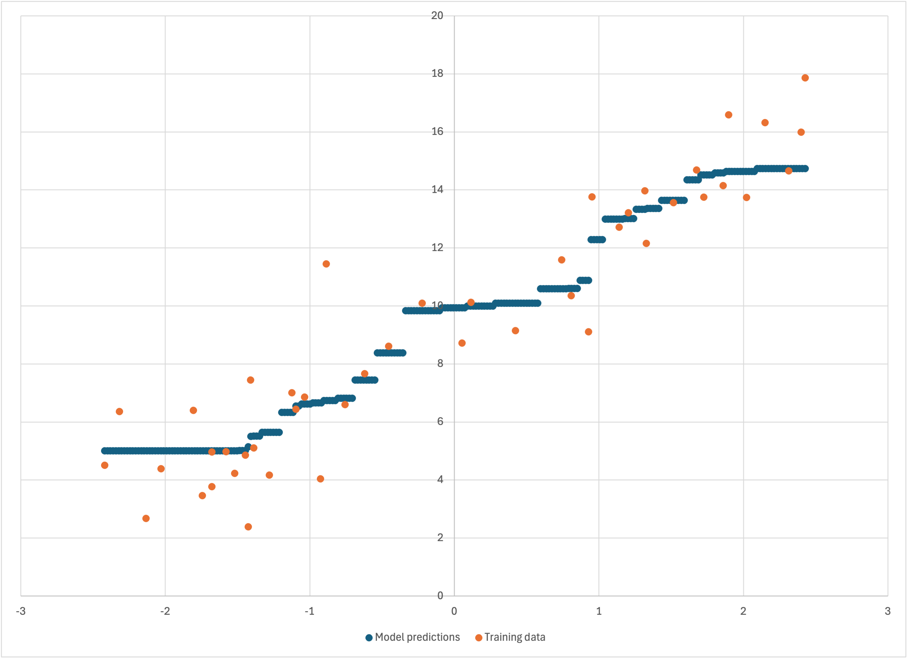
Training data and predictions for the examples without a missing feature value
that Bear has modeled these similarly to the datasets above without missing feature values.
Note that my libraries automatically handle text files that are compressed with gzip. All that you need to do is specify a filename that ends in .gz, and it will all happen automagically. The command gzcat is a useful analog of cat for such files. Note that Bear always saves its model file in compressed format.
If you have followed along with (and hopefully enjoyed) all of the above, then feel free to move on to the intermediate tutorial.
© 2022–2024 John Costella