If you have not worked through the simple tutorial and the intermediate tutorial, I strongly recommend that you work through them first.
In the initial release of Bear I showed that by processing the MNIST images into pyramids of images, diff images, and edges, and extracting the JPEG DCT coefficients of those three pyramids of images, Bear was able to classify the MNIST database with over 98% accuracy with only five minutes of training.
In May 2023 I thought I had found a good generalization of the image pre-processing phase, which I dubbed “Convolutional Bear,” by analogy with Convolutional Neural Networks. However, by the end of May I proved to myself that this initial attempt was wrong.
I am currently working on a correct formulation of Convolutional Bear, which I plan to release in early 2024. In the mean time I have removed all the MNIST programs and tutorials from this site, as superseded.
The MNIST database is the classic test for computer vision algorithms. Here are some references:
The data is on Yann’s page, but others have made it easier to ingest. I have used Joseph Redmon’s version:
Check back in 2024 to see how Convolutional Bear classifies this database.
In the simple and intermediate tutorials I talked about the “weight” of a given Bear model, and promised to make that concrete in this tutorial. That’s what I’ll now do.
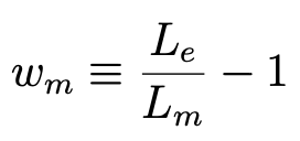
When Bear constructs a model m, it computes the loss Lm based on its predictions of the labels for the training examples, according to the specified loss function (by default, MSE). It then computes the “weight” wm for that model m to be

Definition of the weight of a given model m
where Le, the loss of the empty model, provides a useful normalization. It subtracts 1 so that a model that is no better than the empty model gets a weight of zero.
In the intermediate tutorial I explained that Bear uses each model’s weight for two different things:
Use (2) is fine, and I use the weights as defined above.
For use (1) we have two problems.
First, because of my subtraction of 1 above, models that are useless by themselves will by definition have a weight of zero. But we still want to be able to select these models, since a combination of them may be useful.
One solution would be to not subtract 1 at all, so that useless models would have a selection weight of 1. But my intuition is that this would not be optimal. Imagine a case where we have 1,000 features, and 999 of the 1,000 elementary models happen to be useless, with the other one having a very good weight—say, 9. The total selection weight of 999 for those useless models would swamp the measly selection weight of 9 for the good model, and 99.1% of the time we would never select that good model at all.
Instead, my current solution to this is to add an extra “bonus” selection weight of one unit in total, shared between all of the models that have been created so far. So for my example above, instead of the useless models collectively having a selection weight of 999, they would instead have a collective selection weight of just 0.999. The good model would have a selection weight of 9.001, so would be selected 90.01% of the time.
Second, consider the case that we create a model from a base and an attachment that is only slightly better than the base. Since it is better, we want to keep this new model. But we now have two very similar models in the mix, which together would now have a little more than double the selection weight of the original base model. Effectively, the original base model has doubled its importance, even though the new model is really only a minor improvement.
My solution to this is to apply Occam’s razor and only give the new model a selection weight equal to the improvement of its weight over that of the base model.
At this time I have shown you two main programs in these tutorials: memory_bear and bear_predict. They are general-purpose, and are convenient if you want to read and write text files. I intend to provide more such programs, such as for Convolutional Bear and Bear AI, in 2024.
These programs are thin wrappers around the actual Bear class that does the work. You are free to roll your own executables to wrap the Bear engine however you like (or you can ask me if I’d consider writing it myself). The API for the Bear class is very simple: apart from some tiny ancillary methods, there are just two main methods that do the work:
Bear sets a default limit of “swappable memory” to three-quarters of total memory, and automatically swaps data stored in this swappable memory out to storage when the limit is hit. This limit can be changed using the -g option in memory_bear. Most (but not all) of the data used by Bear is stored in this swappable memory.
However, this version of Bear is still “mainly in-memory” for the training phase: the input data should fit into memory.
In 2024, after releasing Convolutional Bear and Bear AI, I plan to build a fully distributed, Big Data version of Bear (“Big Bear”) which will be able to stream arbitrary amounts of training data from storage through distributed Bear training engines in a standard map–reduce type of architecture.
Play with Bear. Tell me about any bugs. Tell me all the stupid decisions I made that I will kick myself once you explain them to me, and then buy you a beer for making Bear that much better.
Please leave me this feedback on Bear’s Facebook page (really, where did you think I was going to put it?).
Happy Bear-wrangling!
© 2023–2024 John Costella